Monitoring Cell Cycle Dynamics During Stem Cell Differentiation Using the scanR System’s TruAI™ Deep-Learning Technology
Introduction
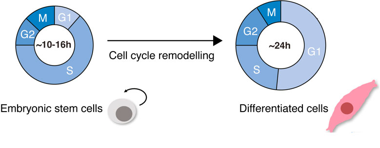
During early mammalian development, embryonic stem cells (ESC) undergo cellular specification and give rise to all the embryonic germ layers, which ultimately generate the multitude of cell types in the adult organism. ESCs are characterized by their incredible ability to self-renew and proliferate, having short division cycles due to truncated GAP phases (G1 and G2). During cellular differentiation, hallmark cellular events happen: cells change their morphology, growing about ten times their size, changing their nucleus-to-cytoplasmic ratio and becoming flat and elongated; fate-specific gene expression programs are activated and global chromatin modifications occur. Importantly, the cell cycle slows down. Differentiated, somatic cells have long G1- and G2-phases, tight checkpoint control, and well-regulated division cycles (Padgett and Santos 2020) (Figure 1).
Cell cycle remodeling is not just a phenomenon that happens in ESC differentiation. Changes in cell cycle dynamics happen frequently in biology; for example, when cells undergo regeneration after viral infections or during malignancy. Studying how cell cycle dynamics change in the context of cellular differentiation is therefore important in understanding potentially conserved mechanisms of cell cycle control and will have an impact on our understanding of the balance between health and disease states.
The changes during differentiation can be monitored in single cells by measuring the activity of genetically encoded proteins involved at different stages of the cell cycle (Araujo et al. 2016; Sakaue-Sawano et al. 2008). One such sensor is the fluorescent ubiquitination-based cell cycle indicator FUCCI(CA), developed by Miyawaki and colleagues (Sakaue-Sawano et al. 2017), which monitors the degradation of Cdt1 and Geminin, two important cell cycle proteins, producing a sharp triple color-distinct separation of the G1, S, and G2 phases (red, green, and yellow) that can be observed in the YFP and mCherry channels of a microscope (Figure 2).
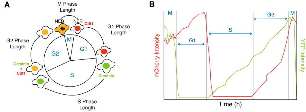
Figure 2. Measuring G1, S, G2 and M-phases of the cell cycle using the FUCCI(CA) sensor. (A) Schematic of the FUCCI(CA) sensor. (B) Example traces of G1, S, G2 and M-phase duration based on expression levels of Cdt1 (mCherry channel) and Geminin (YFP channel).
However, monitoring cell cycle dynamics during cell differentiation presents both imaging and data-analysis challenges. Long-term live cell imaging over days requires a stable temperature and CO2 control, gentle illumination to minimize phototoxicity, and robust autofocus routines to ensure good-quality images during the whole time-lapse process.
For the analysis, the biggest challenge is the segmentation and subsequent tracking of single cells at low fluorescence intensities and high-confluency conditions while the ESCs are moving, dividing, and dramatically changing their shape during differentiation.
All these challenges can be overcome with the Olympus high-content epifluorescence scanR microscope, equipped with a cellVivo incubator, Z-drift compensation (ZDC) hardware for autofocusing, TruAI™ deep-learning technology for segmentation, and a kinetic module for tracking.
Objectives
In this application note, we show that applying TruAI technology can significantly improve detection and tracking of single ESCs through long-term imaging based on the FUCCI(CA) sensor. This is particularly powerful with cells that do not have a nuclear marker for tracking, avoiding unnecessary illumination and phototoxicity.
To achieve this, TruAI technology is used to generate a deep neural network (DNN) model that can robustly identify the position of pluripotent ESCs and differentiated cells at all time points, even when the fluorescence intensity is very weak. This enables robust monitoring of G1, S, and G2 phases of cell populations over time. Subsequently, by applying the scanR kinetic module, we can track thousands of cells, evaluate their traces for long periods of time, and gain quantitative dynamic information on cell cycle changes at the single cell level.
To demonstrate the versatility of the scanR system as a research tool, all the data shown, including graphs, scatter plots, object galleries, tracks, and kinetic traces, are generated using only the scanR software.
Experimental Setup
H1 human embryonic stem (hESC) cells expressing the FUCCI(CA) sensor are treated with 50 ng/ml of bone morphogenic protein 4 (BMP4) to drive differentiation into the mesendoderm lineage. These H1 cells are then imaged using the scanR microscope with a 10X UPLANSAPO lens in the mCherry and YFP channels every 15 minutes for 6 days.
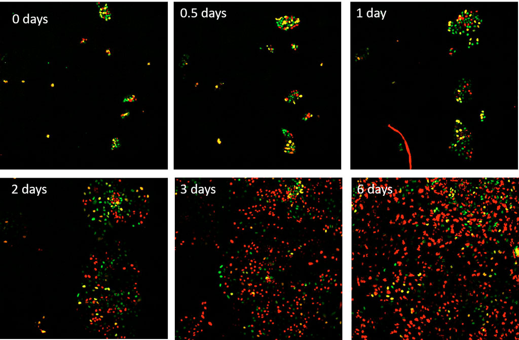
Figure 3. Time series over 6 days of hESC H1 cells expressing the FUCCI(CA) sensor, which were stimulated with BMP4 at the start of imaging. Red, green, and yellow correspond to the G1, S, and G2 phases respectively.
Developing a DNN to Detect Cells for Life Cell Imaging Conditions
A single cell expressing the FUCCI(CA) sensor may exhibit strong variations in fluorescence intensity when monitored over several days. In particular, the total intensity can be very low in the transition from G1 to the S phase (Figure 2b). This can cause tracking algorithms to fail as tracks break at the time points in which the cells are difficult to be detected.
To achieve cell tracking over several days for the largest number of cells possible, a DNN model capable of detecting cells at very weak intensities needs to be developed. In a previous white paper, we showed that this is possible by using pairs of images of long exposure and intense illumination of fluorescent cells versus short exposure and weak illumination (Woerdemann 2020). Briefly, the long exposure images are used for segmentation of cells and a mask is generated. This mask is used as ground truth to train the DNN model to detect cells in the low exposure levels.
Alternatively, the DNN model can be trained by performing manual annotations in the dataset to be analyzed. For this task, Olympus’ cellSens™ software can be used. DNN models developed in cellSens software can be imported into the scanR software. In this application note, we used the latter manual method and provided in the order of hundreds of annotations of cells of varying intensities at different time points to train the DNN model.
Segmentation: Comparison of TruAI Deep-Learning Technology vs Classical Methods
Once developed, the DNN model is applied to the individual mCherry and YFP fluorescence channels. This creates a pixel AI probability map for each channel. The higher the AI probability in a pixel, the higher the confidence that the pixel belongs to a cell. Subsequently, the AI probability maps of both channels are summed, and segmentation is performed by applying an intensity threshold to this summation (Figure 4e and 4f).
To compare the results with classical methods, the mCherry and YFP fluorescence channels are background corrected using a rolling ball algorithm, summed, and the summation is segmented using an intensity threshold (Figure 4c) or an edge detection method (Figure 4d). All the image processing steps described above are conducted on scanR analysis software.
The statistical tools of the scanR system are used to create Table 1, in which results are referred to one single field of view over a period of 6 days.
Table 1. Comparison of number of cells segmented per method
| Time points | Segmentation methods | ||
|---|---|---|---|
| Intensity threshold | Edge detector | TruAI technology | |
| 0 h | 78 | 103 | 93 |
| 24 h | 209 | 188 | 240 |
| 48 h | 421 | 281 | 475 |
| 72 h | 847 | 654 | 986 |
| 96 h | 1480 | 1330 | 1590 |
| 160 h | 1340 | 1460 | 1610 |
|
Summation of all frames
0–160 h | 504131 | 573179 | 659199 |
A simple comparison of the fluorescence image against the AI probability image (Figure 4a and 4b) reveals that the TruAI approach has a higher sensitivity while detecting all types of cells. This is supported by the results summarized in Table 1 along with the whole time lapse. The classical intensity threshold method fails to detect weak fluorescent cells and to determine their correct shape (Figure 4c). The edge detection method improves the contour of the detected cells, but still misses many dim cells (Figure 4d). TruAI deep-learning technology reliably detects dim cells, and their boundaries are well defined (Figures 4e and 4f).
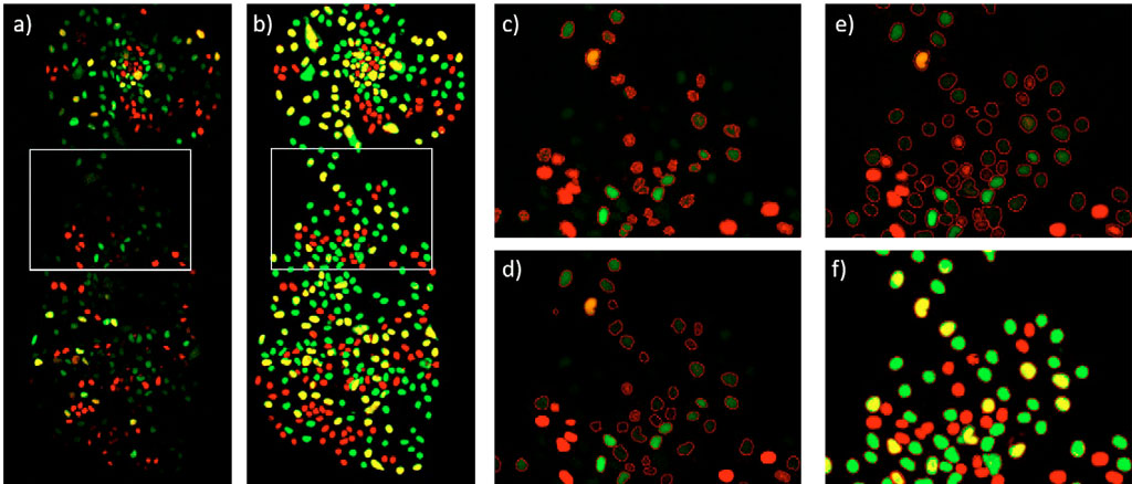
Figure 4: ESC cell colony at time point 48 h. a) mCherry (red, G1 phase) and YFP (green, S phase) fluorescence channels. The G2 phase is seen as a combination of mCherry and YFP (yellow). b) TruAI probability in the mCherry (red) and YFP (green). Cells with high AI probability in both channels are displayed in yellow. c) Segmentation using an intensity threshold in the summation of the mCherry and YFP fluorescence channels d) Segmentation using an edge detector in the summation of the mCherry and YFP fluorescence channels e) Segmentation in the summation of the TruAI probability intensities, overlaid with the fluorescence image f) same as e) but overlaid with the TruAI probability.
Analysis of Cell Populations Over Time
The mCherry and YFP intensities of segmented cells using TruAI technology are displayed in a scatter plot at different time intervals (Figure 5). Cells only having mCherry intensity correspond to the G1 phase, cells exhibiting only YFP intensity correspond to the S phase, and cells having intensities in both channels corresponds to cells in the G2 state. Figure 5 shows that at early times most of cells are in the S state, whereas at later times most of the cells are in the G1 state. This population shift matches with the cell cycle profiles expected for pluripotent and differentiated cells, respectively (Figure 1).
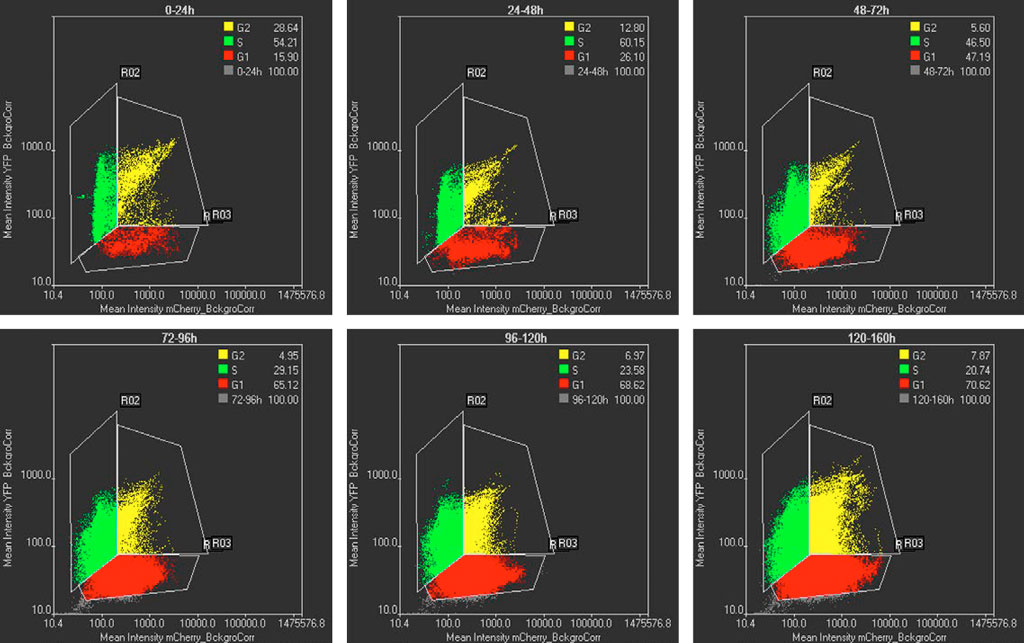
Figure 5: Scatterplots of mCherry vs YFP intensities at different time intervals. Each dot in the scatterplot represents a segmented cell by TruAI technology. G1, S, and G2 cells are represented in red, green, and yellow respectively. The % of the G1-S-G2 populations are shown in the inserts. The time intervals are shown at the top of each graph.
Cell Tracking: Comparison of TruAI Technology vs Classical Methods
Cells segmented with the three methods (intensity threshold, edge detector, and TruAI technology) were tracked using the same tracking settings of the scanR kinetic module. The statistical tools of the scanR system are used to create Table 2, in which results are referred to one single field of view over a period of 6 days.
Table 2. Comparison of number of cells tracked per method
| Time points | Number of cells tracked | ||
|---|---|---|---|
| Intensity threshold | Edge detector | TruAI technology | |
| 24 h or more | 302 | 1030 | 1965 |
| 48 h or more | 16 | 126 | 426 |
| 72 h or more | 0 | 27 | 72 |
| 96 h or more | 0 | 0 | 5 |
The table shows that using TruAI technology for segmentation clearly improves the subsequent tracking results. For this data set, considering an average number of 200 cells per field of view at time 24 h (Table 1), more than 70 cells can be tracked over 3 days and it is even possible to track cells for 4 days or longer. The ability to track this high number of cells for such long periods of time is important because it enables the study of cell cycle dynamics over many cell divisions in a statistically meaningful manner.
Analysis of Cellular Tracks
For each track generated by the scanR system, a wide range of parameters can be extracted.
- To identify the longest tracks, the parameter “lifetime” can be plotted in a histogram, and a gate for tracks over 24 h can be created (Figure 6a).
- To filter the tracks further, the parameters “First (time)” and “Last (time)” can be represented in a scatter plot (Figure 6b). This can help us identify the cells only tracked during the first days (ESC cells with short cycle times), the cells tracked only in the last days (differentiated cells with long cell cycle times) and the cells that have been tracked from the beginning till the end of the time lapse (cells in which the differentiation process is monitored). Once these tracks are identified the intensities of mCherry and YFP can be plotted over time to gain quantitative information on the cell cycle dynamics (Figure 6 c, d, e).
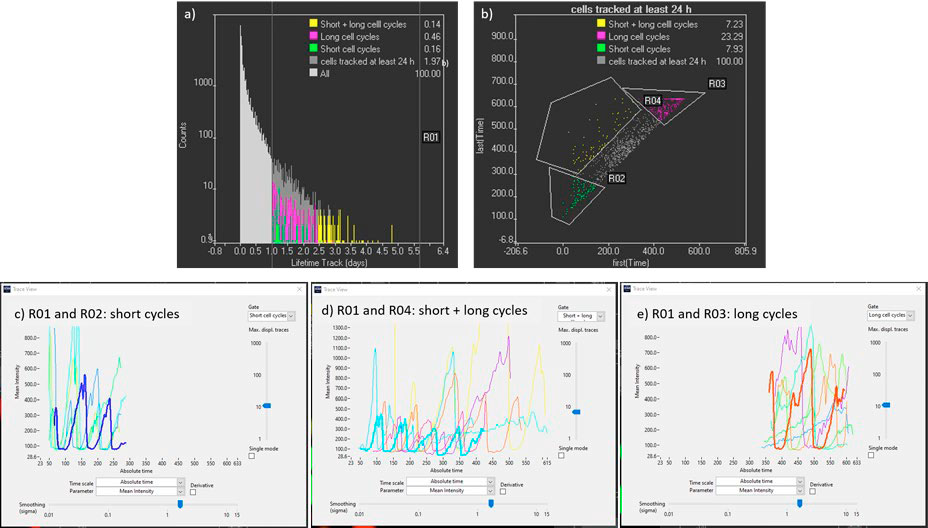
Figure 6. a) Track lifetime histogram used to filter long tracks (R01). b) Scatter plot with initial and final time point of the tracks to identify cells tracked from the beginning till the end of the time lapse (R01 and R04). c), d), and e) Kinetic traces of mCherry cells tracked more than 24 h with early starting and ending points, with early starting points and late ending points, and with late starting and ending points respectively. Time points are spaced 15 minutes apart.
From Figure 6c to 6e, it is observed that mCherry (G1 state) signal duration increases with time, from approximately 2 hours for ESC cells to 24 h once the cells have differentiated. For the in-depth analysis of the cell cycle dynamics, it is possible to select tracks of region R01 and R04, in which the transformation of ESC to differentiated cells is monitored over four or more cell divisions (Figure 6d).
Figure 7 represents the monitoring of one ESC cell undergoing differentiation over five cell cycles. In Figure 7a, the position of the ESC in its colony is shown at time point 52 (13 h), along with its track up to time point 422 (105 h). In Figure 7b, a snapshot at time 280 (70 h) is shown. Note the intensity of this cell is extremely weak and it went undetected using the classical methods. In Figure 7c, the same snapshot is shown, but with the TruAI probability image. The probability intensity of the tracked cell is as high as for the rest of the cells. Figures 7d and 7e represent a gallery of the tracked cell at time points every 15 minutes for fluorescence and TruAI probability respectively. Note that when finishing the G1 phase (red color), the total intensity is always very weak. Figure 7f represents the mCherry (top) and YFP (bottom) fluorescence intensity oscillations from which the cell cycle periods of G1, S, G2, and M states can be extracted.
From these data, we observe that this particular cell spends increased time in the G1 state and reduced time in S and G2 phases as time progresses. The M state is always very short; its exact position appears like a dip in the mCherry signal and as a drastic decay in the YFP signal.
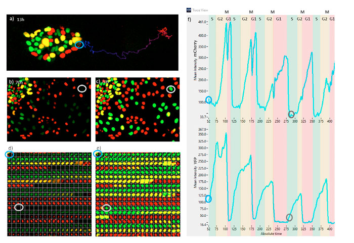
Figure 7. a) Fluorescence snapshot at the 13 h time point. b) Fluorescence snapshot at the 70 h time point. c) TruAI snapshot at 70 h. d) Fluorescence time-lapse sequence of the tracked cell at 15-minute intervals. e) TruAI time-lapse sequence of the tracked cell at 15-minute intervals. f) Fluorescence traces of mCherry and YFP of the tracked cell indicating the periods of the different cell cycle phases. Time steps correspond to 15 min. Blue and gray callouts in a–f indicate the same cell at 13 h or 70 h, respectively.
Conclusion
This novel deep-learning approach of analyzing cell cycle dynamics during ESC differentiation combined with the kinetic module of the scanR high-content screening system enables the acquisition of highly reproducible, quantitative, and statistically meaningful data on how cell cycle dynamics change in single cells during differentiation. Thousands of cells changing in shape and morphology can be recognized and tracked over days of differentiation using fluorescence measurements. This is a powerful tool to study cell cycle dynamics in early development and reprogramming, as well as in cells undergoing cellular transformation (malignancy) where cell cycle regulation takes central stage.
References
Padgett, J., and Santos, S.D.M. 2020. “From clocks to dominoes: lessons on cell cycle remodeling from embryonic stem cells.” FEBS Letters. 10.1002/1873-3468.13862.
Araujo, A.R., Gelens, L., Sheriff, R.S.M., and Santos, S.D.M. 2016. “Positive feedback keeps duration of mitosis temporally insulated from upstream cell cycle events.” Molecular Cell 64, 362–375.
Sakaue-Sawano et al. 2008. “Visualizing Spatiotemporal Dynamics of Multicellular Cell-Cycle Progression.” Cell 132, 487–498.
Sakaue-Sawano et al. 2017. “Genetically Encoded Tools for Optical Dissection of the Mammalian Cell Cycle.” Molecular Cell 68, 626–640.
Woerdemann, M., and Genenger, M. 2020. “TruAI™ Technology with Deep Learning for Quantitative Analysis of Fluorescent Cells with Ultra-Low Light Exposure.” Olympus Application Note. www.olympus-lifescience.com/en/resources/white-papers/ultra-low_light_exposure_analysis/
Authors
Joe Padgett and Silvia Santos
Quantitative Stem Cell Biology Lab, The Francis Crick Institute, 1 Midland Road, NW1 1AT, London, UK
Manoel Veiga Gutierrez
Olympus Soft Imaging Solutions GmbH, Johann-Krane-Weg 39, 48149 Muenster, Germany
Products related to this application
Sorry, this page is not
available in your country.