Digital Images Interpolation and Image Rotation

Geometrical Transformation - Java Tutorial

The geometric transformation of digital images is an important tool for modifying the spatial relationships between pixels in an image, and has become an essential element for the post-processing of digital images. This interactive tutorial explores the basic properties of geometric transformation, and how the algorithms involved in the mechanism of transformation can influence the final appearance as well as the information content of the transformed image.

The tutorial initializes with a randomly selected digital image of a specimen appearing in the left-hand window entitled Specimen Image. Each specimen name includes, in parentheses, an abbreviation designating the contrast mechanism employed in obtaining the image. The following nomenclature is used: (FL), fluorescence; (BF), brightfield; (DF), darkfield; (PC), phase contrast; (DIC), differential interference contrast (Nomarski); (HMC), Hoffman modulation contrast; and (POL), polarized light. Visitors will note that specimens captured using the various techniques available in optical microscopy behave differently during image processing in the tutorial.

Positioned to the right of the Specimen Image window is a Rotated Image window that displays the captured image at various angles of rotation. The image rotation angle is adjustable with the Angle of Rotation slider. Several mechanisms of image filtering can be individually selected by utilizing the Filtering Method pull-down menu. To operate the tutorial, select an image from the Choose A Specimen pull-down menu, and vary the angle of rotation using either the Angle of Rotation slider or the blue arrow buttons appearing to the left and right of the slider. The current rotation angle is displayed (measured in degrees from the vertical axis) directly above the slider control bar. When the mouse cursor is rolled over the digital image appearing in the Specimen Image window, a small white circle representing the image pivot point will appear on the image. Clicking the mouse cursor anywhere within the boundaries of the specimen image will move the pivot point to that new location, and will automatically shift the rotational origin of the rotated image to the new center of rotation. An enlarged view of the specimen (and the algorithm interpolation results) is available with the Zoom Factor slider. The zoom control can be utilized to enlarge the Rotated Image view by increments of 2x, 4x, or 6x in order to more clearly visualize pixel color changes, distortion, and fluctuation in brightness values as the image is transformed. Visitors should examine the effects of the various filtering methods on the visual quality of the rotated image while varying the angle of rotation with the slider.

Digital images captured in the microscope must often be rotated in order to perform measurements on the specimen and/or to produce the desired orientation for viewing, display, or printing. A majority of the professional image editing software packages provide filtering options for geometric image transformations, and it is important to understand how the application of various transformation methods can affect the visual quality of the transformed image.

The basis for geometric transformation of a digital image, as in related image processing techniques, is an operation that transforms the original image (source) into the transformed image (destination). In the case of rotation, this means applying a function that maps each point in the source image to its corresponding point in the destination image. This type of algorithm is not used in practice, however, because the rotated destination image will often contain unwanted gaps or holes because (in many cases) it requires a greater number of pixels than the source to properly display the rotation.

A simple solution to this problem is to perform an inverse-transformation from each pixel in the rotated image to a corresponding pixel in the source image. This solution has the advantage of ensuring that each pixel in the destination image will have a corresponding pixel from the source image assigned to it. Unfortunately, the calculated coordinates for the location of the pixel in the source image will only rarely be integers. The result is that the calculated pixel location often lies in an area between two or more pixels in the original image. A number of methods are available to deal with this problem. The simplest approach involves the Nearest Neighbor algorithm, which operates by truncating the calculated coordinates so that the fractional part of the address is discarded. Another very similar approach, the Rounded Nearest Neighbor method, rounds the calculated coordinate values to the nearest integer value. Either method introduces a small degree of error that will distort the rotated image at certain angles. In some cases this distortion is acceptable, but better results can usually be obtained by interpolating brightness values over a small neighborhood of pixels, with the added expense of more detailed computations. Additionally, interpolation can result in a loss of accuracy, since interpolated pixel brightness values are not the same as those from the original image.

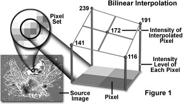
The method of bilinear interpolation employs a four-pixel neighborhood (2 × 2 array, or a pixel set) surrounding the calculated pixel address to obtain a new transformed pixel value. Bilinear interpolation involves computing a weighted average of the pixel set brightness values based on the fractional part of the calculated pixel's address, as illustrated in Figure 1 for an array of pixels having brightness values of 116, 141, 191, and 239.

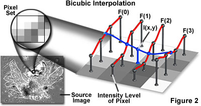
Similarly, the method of bicubic interpolation (illustrated in Figure 2) involves fitting a series of cubic polynomials to the brightness values contained in the 4 × 4 array of pixels surrounding the calculated address. First, four cubic polynomials F(i), i = 0, 1, 2, 3, are fit to the control points in the y-direction (the choice of starting direction is actually arbitrary). Next, the fractional part of the calculated pixel's address in the y-direction is used to fit another cubic polynomial in the x-direction, based on the interpolated brightness values that lie on the curves F(i), i = 0, ..., 3. Substituting the fractional part of the calculated pixel's address in the x-direction into the resulting cubic polynomial then yields the interpolated pixel's brightness value.

The choice of polynomial type utilized in the bicubic interpolation algorithm can have a significant impact on the accuracy and visual quality of the interpolated image. Splines are piecewise polynomial functions that are often used in bicubic interpolation algorithms. One requirement of splines used for bicubic interpolation is that they should always interpolate the brightness values of the pixels contained in the 4 × 4 control grid. Since many types of spline have control parameters that are subject to the choice of the programmer, reproducibility becomes an issue when employing bicubic interpolation algorithms.

In summary, nearest neighbor methods preserve pixel values at the expense of aliasing of lines and edges, while interpolation methods preserve lines and edges but at the expense of altering pixel values. The choice of method depends primarily on the type of information desired for a particular application (e.g., measurement of dimensions or of density).

In the tutorial, distortion produced by the nearest neighbor methods can be clearly seen in all of the example images, although it is especially noticeable in those images having high-spatial-frequency detail. Included with the two nearest neighbor methods is an option to apply a low-pass filter algorithm to the rotated image (the Box Average Filter checkbox). Checking this option will remove some of the distortion at the expense of substantially blurring the transformed image. Superior visual quality can be seen with the methods of bilinear and bicubic interpolation.