During the examination and digital recording of multiply labeled fluorescent specimens, two or more of the emission signals can often overlap in the final image due to their close proximity within the microscopic structure. This effect is known as colocalization and usually occurs when fluorescently labeled molecules bind to targets that lie in very close or identical spatial positions. The application of highly specific modern synthetic fluorophores and classical immunofluorescence techniques, coupled with the precision optical sections and digital image processing horsepower afforded by confocal and multiphoton microscopy, has dramatically improved the ability to detect colocalization in biological specimens.
Colocalization, in a biological manifestation, is defined by the presence of two or more different molecules residing at the same physical location in a specimen. Within the context of a tissue section, individual cell, or sub-cellular organelle viewed in the microscope, colocalization may indicate that the molecules are attached to the same receptor, while in the context of digital imaging, the term refers to colors emitted by fluorescent molecules sharing the same pixel in the image. In confocal microscopy, specimens are recorded as a digital image composed of a multi-dimensional array containing many volume elements termed voxels that represent three-dimensional pixels. The size of a voxel (or detection volume) is determined by the numerical aperture of the objective, the illumination wavelength, and the confocal detector pinhole diameter. Thus, the colocalization of two fluorescent probes in a specimen, such as Alexa Fluor 488 having green emission and Cy3 with orange-red emission, is represented in the image by pixels containing both red and green color contributions (often producing various shades of orange and yellow).
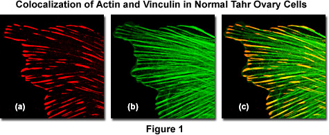
As an example, the image sequence presented in Figure 1 illustrates colocalization in the lateral optical plane (x-y axis on a laser scanning confocal microscope) of the cytoskeletal protein actin with vinculin, a protein associated with focal adhesion and adherens junctions. These complexes serve as nucleation sites for actin filaments and as crosslinkers between the external medium, plasma membrane, and actin cytoskeleton. Figure 1(a) is the scan collected from a detector channel filtered for the emission spectrum of Alexa Fluor 568 (vinculin) when excited with a 543-nanometer helium-neon laser, while Figure 1(b) is the channel filtered to gather fluorescence emission from Alexa Fluor 488 (filamentous actin) excited with an argon-ion laser at 488 nanometers. Digitally combining the two images (Figure 1(c)) reveals colocalization of the two fluorescence signals at the termini of filamentous actin fibers.
It is important to note that colocalization does not refer to the likelihood that fluorophores with similar emission spectra will appear in the same pixel set in the composite image. Accurate colocalization analysis is only possible if the fluorescence emission spectra are sufficiently well separated between fluorophores and the correct filter sets (or spectral slit widths) are using during the acquisition sequence. If spectral bleed-through artifacts are present because of a high degree of spectral overlap between the fluorophore emission spectra, or due to the use of incorrect filter combinations, colocalization measurements will be meaningless. To avoid artifacts, the fluorophores must be carefully matched to the power spectrum of the illumination source (laser lines in confocal microscopy) to obtain the maximum excitation efficiency while still maintaining a useful degree of separation between emission wavelengths. In most cases, the judicious choice of fluorophores for colocalization analysis is paramount in obtaining satisfactory results.
A comparison of spectral overlap for a series of Alexa Fluor dye combinations that are potentially useful in colocalization experiments is presented in Figure 2. All of the emission spectra are normalized for comparison, and the overlap regions are indicated by gray shading. In Figure 2(a), the emission spectra for the green fluorescent Alexa Fluor 488 and yellow-orange fluorescent Alexa Fluor 555 dyes indicate clear separation of the peak wavelengths, which are also easily distinguished by the human eye. However, the moderate level of spectral overlap (gray shaded area) illustrates that there is a considerable amount of emission from Alexa Fluor 488 at the peak emission wavelength of Alexa Fluor 555 (denoted by a black line running from the emission peak to the abscissa). This high level of signal bleed-through renders separation of the probes difficult in situations where the fluorescence emission intensity of Alexa Fluor 488 is significantly greater than that of Alexa Fluor 555, which can occur due to a number of factors including large differences in the fluorophore target population. As a result, the combination of these probes should either be avoided in colocalization experiments, or used only when images are acquired in multitracking confocal mode to reduce or eliminate bleed-through.
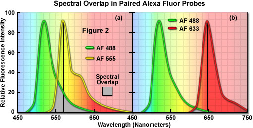
The spectral overlap between Alexa Fluor probes decreases as the bandwidth between emission maxima increases, as illustrated in Figure 2(b). In this case, Alexa Fluor 488 and deep red fluorescent Alexa Fluor 633 demonstrate a significantly reduced level of overlap when compared to Figure 2(a). Both dyes are easily distinguishable to the human eye and the low degree of spectral overlap should yield good results with minimal bleed-through in colocalization experiments, provided the concentrations of each probe are similar (note that the deep red fluorescence of Alexa Fluor 633 may be difficult to visualize through the microscope eyepieces at low concentrations). Alexa Fluor 633 is most efficiently excited by the 633-nanometer line of a red helium-neon laser, but can also be used with the 594-nanometer line of a yellow helium-neon laser. Perhaps the best spectral separation in visible-light emitting Alexa Fluor dyes is the combination of Alexa Fluor 488 and Alexa Fluor 647 (not illustrated). There is virtually no spectral overlap between these dyes and bleed-through artifacts should be absent, even in specimens containing excessive levels Alexa Fluor 488. Fluorescent probes with these characteristics are ideal candidates for colocalization investigations on confocal microscopes equipped with the appropriate lasers.
The ability to determine colocalization in a confocal microscope is limited by the resolution of the optical system and the wavelength of light used to illuminate the specimen. Widefield fluorescence and confocal microscopes have a theoretical resolution of approximately 200 nanometers (0.2 micrometer), but in practice, this number drops to a value between 400 and 600 nanometers for a variety of reasons, including misalignment of the microscope, refractive index fluctuations, optical aberrations, and improper specimen preparation. In almost all cases, however, the optical resolution limit of a perfectly tuned confocal microscope is not sufficient to determine whether two fluorescent molecules are attached to a single target, or whether they even reside within the same organelle. Many experimental protocols are designed around highly specific synthetic probes or antibodies targeting localized and well-defined cellular structures that are readily discriminated. Others produce specimens with regions that display a high degree of overlap between probes.
For specimens that are less than 5 micrometers in thickness, such as adherent cells or very thin tissue sections, quantitative colocalization analysis is often possible in a conventional widefield fluorescence microscope. However, for thicker specimens, images should be recorded as optical sections of limited axial dimension to determine if seemingly colocalized fluorophores actually reside in the same lateral focal plane or whether they are vertically superimposed over each other along the microscope z-axis. The colocalization analysis of fluorophores in thick specimens should be conducted by obtaining thin optical sections using either laser scanning or spinning disk confocal or multiphoton microscopy. Multiphoton instruments are often able to excite both fluorophores in dual labeled specimens with a single near-infrared laser spectral line in a highly defined volume at the focal point of the objective. This unique feature limits fluorescence emission to fluorophores residing only in the focal plane, which dramatically reduces photobleaching artifacts and background noise.
Software Analysis of Colocalization
The degree of fluorophore colocalization in a specimen is measured by comparing color values for the equivalent pixel position in each of the acquired images. The first step in the analysis process involves display of the image upon which the colocalization measurements will be performed, either as a composite derived from two independent channel single-wavelength acquisitions (the preferred technique) or a multiply labeled specimen acquired as a single image. When examining specimens having more than two labels, only two pseudocolors are processed during a single calculation, but all pseudocolor permutations can subsequently be selected as pairs for colocalization analysis. Typically, red-green pairs are selected for confocal fluorescence due to the traditional use of argon-ion, krypton-argon, and helium-neon lasers, which have spectral lines capable of efficiently exciting fluorophores that absorb strongly in the blue and green regions. In addition, the human eye is more sensitive to hues in the green and red color groups.
Graphical display for colocalization analysis of the pseudocolored specimen image is conveniently represented by a scatterplot (sometimes referred to as a fluorogram), which correlates the relationship or association between two sets of data. A scatterplot graphs the intensity of one pseudocolor (or channel) versus another for each pixel in the image, or a selected region of interest, on a two-dimensional histogram (see Figures 3 and 4). One channel (usually green) is graphed along the x-axis, while the other (usually red) is plotted on the y-axis with intensities ranging from 0 to 255 on both the abscissa and ordinate. Thus, every pixel of the composite image is characterized by a pair of intensities distinguished as coordinates in a Cartesian system. Analysis of the distribution pattern generated by the intensity pairs enables identification of fluorophore colocalization, as well as background discrimination, bleed-through, photobleaching, and lack of registration between the individual channels.
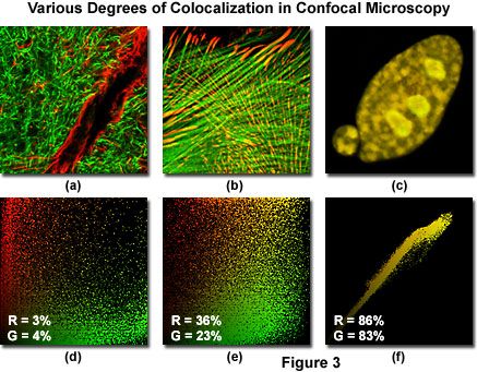
Figure 3 illustrates three dual channel confocal microscopy optical section image planes (pseudocolored red and green) from specimens having varying degrees of fluorophore colocalization, along with their corresponding scatterplots. Pixels in each channel having very low intensity are located near the origin (0,0) of the scatterplot, while brighter pixels are dispersed farther away and across the entire graph. In a scatterplot that correlates red and green channels, the pure red and green pixels tend to cluster near the axes of the plot, while colocalized pixels, if present, appear colored with orange and yellow hues (depending upon the degree of colocalization), and fall near the center (x = y) and upper right-hand corner of the scatterplot.
The specimens presented in Figure 3 include a rat brain hippocampus coronal thick section labeled with Alexa Fluor 488 (neurofilaments) and Alexa Fluor 568 (glial fibrillary acidic protein; GFAP, Figure 3(a)). An Indian Muntjac deer skin fibroblast cell stained with Alexa Fluor 568 targeting vinculin and Alexa Fluor 488 conjugated to phalloidin (filamentous actin) is illustrated in Figure 3(b), while a rabbit kidney epithelial cell (RK-13 line) co-expressing the fluorescent proteins, DsRed and EYFP, localized to the nucleus, is depicted in Figure 3(c). The associated scatterplots are positioned directly beneath the specimen image (for example, Figure 3(d) is the scatterplot for Figure 3(a)), and the degree of colocalization for both channels is indicated by white letters and numbers in the lower left-hand corner of each scatterplot. Note the relative lack of colocalization (only a couple percent for both channels) in Figure 3(a), and the progressively higher degrees of colocalization in Figures 3(b) and 3(c), which feature coefficients of approximately 30 and 85 percent, respectively.
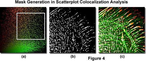
Scatterplot analysis of fluorophore colocalization using typical software provided by confocal microscope and aftermarket imaging program manufacturers is outlined by the sequence of images displayed in Figure 4, which were generated using Indian Muntjac fibroblast cells stained with Alexa Fluor 568 (vinculin; red channel) and Alexa Fluor 488 (filamentous actin; green channel). A region of interest is selected for analysis in the scatterplot, as denoted by the white rectangle in Figure 4(a). This region sets the threshold levels of signal that will be included in the analysis performed by most colocalization software programs.
The vertical and horizontal edges outlining the area of interest should be aligned to exclude background signal, which is clustered along the x and y-axes of the scatterplot. Only the signal arising from pixels included within the boundaries of the selected region is analyzed in the estimation of colocalization. Overlapping pixel regions in the specimen are easily converted into a colocalization binary threshold mask (Figure 4(b)), which can be superimposed on the image (Figure 4(c)) as a colocalization map. The threshold portion of map illustrated in Figure 4(c) shows colocalized areas in white, but this color can be readily changed with most software applications to another color that produces a higher degree of contrast relative to the original pseudocolors.
As discussed above, a quantitative assessment of fluorophore colocalization in confocal optical sections can be obtained using the information obtained from scatterplots and selected regions of interest. Several values are generated using information from the entire scatterplot, while others are derived from pixel values contained within a selected region of interest. Among the variables used to analyze the entire scatterplot is Pearson's correlation coefficient (R(r)), which is one of the standard techniques applied in pattern recognition for matching one image to another in order to describe the degree of overlap between the two patterns. Pearson's correlation coefficient is calculated according to the equation:
 | (1) |
where S1 is the signal intensity of pixels in the first channel and S2 is the signal intensity of pixels in the second channel. The values S1(average) and S2(average) are the average values of pixels in the first and second channel, respectively. In Pearson's correlation, the average pixel intensity values are subtracted from the original intensity values. As a result, the value of this coefficient ranges from -1 to 1, with a value of -1 representing a total lack of overlap between pixels from the images, and a value of 1 indicating perfect image registration. Pearson's correlation coefficient accounts only for the similarity of shapes between the two images, and does not depend upon image pixel intensity values. When applying this coefficient to colocalization analysis, however, the potentially negative values are difficult to interpret, requiring another approach to clarify analysis results.
A simpler technique often employed to calculate an alternative correlation coefficient involves eliminating the subtraction of average pixel intensity values from the original intensities. Defined formally as the Overlap coefficient (R), this value ranges between 0 and 1 and is not sensitive to intensity variations in the image analysis. The Overlap coefficient is defined as:
 | (2) |
The product of channel intensities in the numerator returns a significant value only when both values belong to a pixel involved in colocalization (if both intensities are greater than zero). As a result, the numerator in equation (2) is proportional to the number of colocalizing pixels. In a similar manner, the denominator of the Overlap equation is proportional to the number of pixels from both components in the image, regardless of whether colocalization is present (Note: the components are defined as the red and green images or the pixel arrays from channel 1 and channel 2, respectively). A major advantage of the Overlap coefficient is its relative insensitivity to differences in signal intensities between various components of an image, which are often produced by fluorochrome concentration fluctuations, photobleaching, quantum efficiency variations, and non-equivalent electronic channel settings.
The most important disadvantage of using the Overlap coefficient is the strong influence of the ratio between the number of image features in each channel. To alleviate this dependency, the Overlap coefficient is divided into two different sub-coefficients, termed k(1) and k(2) in order to express the degree of colocalization as two separate parameters:
 | (3) |
The overlap coefficients, k(1) and k(2), describe the differences in intensities between the channels, with k(1) being sensitive to the differences in the intensity of channel 2 (green signal), while k(2) depends linearly on the intensity of the pixels from channel 1 (red signal). The equations described thus far are able to generate information about the degree of overlap and can account for intensity variations between the color channels. In order to estimate the contribution of one color channel in the colocalized areas of the image to the overall amount of colocalized fluorescence, an additional set of colocalization coefficients, m(1) and m(2), are defined:
 | (4) |
The colocalization coefficient m(1) is employed to describe the contribution from channel 1 to the colocalized area, while the coefficient m(2) is used to describe the same contribution from channel 2. Note that the variable S1(i,coloc) is equal to S1(i) if S2(i) is greater than zero and vice versa for the variable S2(i,coloc). These coefficients are proportional to the amount of fluorescence of the colocalizing fluorophores in each channel of the composite image, relative to the total fluorescence in that channel. Colocalization coefficients m(1) and m(2) can be determined even when the signal intensities in the two image channels have significantly different levels.
A second pair of colocalization coefficients can be calculated for pixel intensity ranges defined by an area of interest delineated on the scatterplot. The coefficient M(1) is utilized to describe the contribution of the channel 1 fluorophore to the colocalized area, while M(2) is used to describe the contribution of the channel 2 fluorophore. These colocalization coefficients are defined as:
 | (5) |
where S1(i,coloc) equals S1(i) if S2(i) lies within the region of interest thresholds (left and right sides of a rectangular ROI) and equals zero if S2(i) represents a pixel outside the threshold levels. Similarly, S2(i,coloc) equals S2(i) if S1(i) lies within the region of interest thresholds (top and bottom sides of a rectangular ROI) and equals zero if S1(i) is outside the region of interest. In other words, for each channel, the numerator represents the sum of all pixel intensities in that channel that also have a component from the other channel, whereas the denominator represents the sum of all intensities from the channel. These coefficients are proportional to the amount of fluorescence of colocalizing objects in each channel of the composite image, relative to the total fluorescence in that channel.
A majority of the colocalization software analysis programs available commercially are able to calculate the parameters described above, including Pearson's correlation coefficient, the total overlap coefficient, as well as the individual k(x), m(x), and M(x) colocalization coefficients. In addition, many programs contain algorithms to apply background subtraction corrections, generate scatterplots of the entire image, and/or perform the calculations using selected regions of interest on single dual channel composite images or optical stacks along the axial plane. The most important data output from these software packages is the colocalization coefficient, which indicates the relative degree of overlap between signals. For example, a colocalization coefficient value of 0.75 for the fluorophore in channel 1 indicates that the ratio for all channel 1 intensities that have a channel 2 component, divided by the sum of all channel 1 intensities, is 75 percent. This is a relatively high degree of colocalization. Likewise, a value of 0.25 for the channel 2 fluorophore indicates a significantly diminished level of colocalization (equal to one-third of the channel 1 fluorophore).
Artifacts and Specimen Considerations in Colocalization Analysis
Among the most important artifacts encountered with colocalization analysis are spectral bleed-through due to emission spectral overlap, autofluorescence (primarily in tissue specimens), and non-specific antibody or synthetic fluorophore staining. Fluorescence resonance energy transfer (FRET) is also a potential artifact with colocalized fluorophores having closely overlapping spectral profiles. Any of these artifacts are capable of producing image pixels that appear yellow or orange, but do not arise from colocalization, when examining specimens labeled with green and red fluorescent probes.
Perhaps the most common problem is the bleed-through of fluorescence intensity when imaging specimens having two or more fluorescent labels. For example, when double labeling with the traditional green and red probes, fluorescein and rhodamine, bleed-through can only be reduced by using optimized fluorescence filter sets, but is never completely eliminated. This effect is due to the fact that these dyes have very broad absorption and emission spectra that exhibit a significant degree of overlap. Thus, excitation of fluorescein using the 488-nanometer spectral line of an argon-ion laser will also produce excitation rhodamine, although to a lesser degree. Furthermore, fluorescein emission will be detected in the photomultiplier channel or widefield filter set reserved for rhodamine, producing pixels that appear yellow or orange even in situations where colocalization is absent. In order to conduct colocalization experiments with these and similar fluorophores, bleed-through artifacts must be completely eliminated.
The problems associated with bleed-through in traditional fluorophores (such as fluorescein and rhodamine) can often be overcome by using newer biologically improved and brighter synthetic probes, such as the Alexa Fluor family or carbocyanine (Cy series) dyes. Many of these specially designed organic molecules exhibit very narrow emission spectra (compared to traditional probes), large extinction coefficients coinciding with arc-discharge lamp and laser spectral lines, improved quantum yields, reduced photobleaching, and less dependence of fluorescence emission on environmental variables. In addition, these advanced probes are available with excitation spectral profiles spanning a bandwidth of approximately 400 nanometers, from the ultraviolet to the near-infrared, ensuring a wide variety of choices to match illumination sources with minimal emission spectral overlap.
Autofluorescence, which is far more pronounced with formaldehyde-fixed tissue specimens, produces artifacts similar in appearance to bleed-through. Excitation of a specimen exhibiting autofluorescence often results in detection of emission in other channels to yield images that appear to have colocalized fluorophores. Excessive background staining by antibodies and synthetic fluorophores can also resemble colocalization in regions where two fluorophores both exhibit high levels of non-specific staining. This artifact can usually be avoided or, at the least, significantly reduced by carefully preparing specimens and monitoring the protocol with proper controls.
Colocalization investigations can only be considered accurate when all bleed-through, autofluorescence, and non-specific fluorescence artifacts have been eliminated. The most effective approach is to employ sequential excitation in the confocal microscope scanning configuration and to collect emission signals with narrow bandpass emission filters (or narrow slit widths for spectral instruments). Simultaneously, single-labeled control specimens should be examined to ensure the complete elimination of bleed-through, and unstained controls can be effective in monitoring autofluorescence. Bleed-through correction software is available for many confocal microscopes to enable correction while images are being captured.
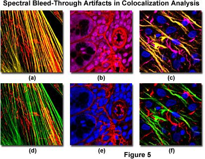
Bleed-through artifacts and their correction in laser scanning confocal microscopy are illustrated in Figure 5 for a variety of specimens. The fibroblast cells presented in Figure 5(a) depict bleed-through of Alexa Fluor 488 (green fluorescence) into the channel intended for MitoTracker Red (red fluorescence) to produce yellow actin filaments when the specimen is scanned simultaneously with argon-ion (488 nanometer spectral line) and green helium-neon (543 nanometer line) lasers. Sequential scanning and detection (Figure 5(d)) eliminates the bleed-through. Likewise, bleed-through in a thick section of mouse intestine (Figure 5(b)) occurs with simultaneous scanning using Cy3 and the nuclear probe, DRAQ5, coupled with green and red helium-neon (633 nanometer line) excitation. Scanning the specimen sequentially (Figure 5(e)) removes the bleed-through artifact that masquerades as colocalization.
In cases where multiply labeled specimens are scanned with more than two lasers, bleed-through artifacts are often observed in several channels, as illustrated in Figures 5(c) and 5(f) for a thick section of rat brain labeled with Alexa Fluor 488 (neurofilaments), Alexa Fluor 568 (GFAP), and DRAQ5 (nuclei). Bleed-through appears in the second and third channels when the specimen is scanned simultaneously with three lasers (Figure 5(c)), indicating the potential for colocalization between the intermediate filaments in this specimen. However, upon initiating sequential scanning and data collection, the filaments appear only in their respective channels (Figure 5(f)), eliminating considerations of fluorophore colocalization in these structures.
Fluorescence resonance energy transfer, which can theoretically measure short distances between two closely positioned fluorophores, is also a potentially useful tool for monitoring colocalization. However, the phenomenon can often lead to artifacts during colocalization analysis unless the specific parameters necessary for FRET are well understood and carefully considered during design of the experiment. Specifically, the investigator should be concerned when using probes that have spectral profiles occupying the same bandwidth, especially in regions where the emission spectrum of the first fluorophore overlaps with the excitation spectrum of the second. Energy transfer in these specimens is manifested in an unexpected decrease in fluorescence emission from the first fluorophore along with a similar unanticipated increase in the emission intensity for the second probe. Interaction between closely associated fluorophores can also result in quenching of the emitted fluorescence signal, depending upon the environmental conditions.
Many of the potential artifacts in colocalization analysis can be circumvented by careful attention to specimen preparation techniques. As discussed above, fluorescent probes should be chosen that have widely separated emission spectral profiles with a minimum of overlap. If possible, choose a green fluorophore that has a narrow emission specimen (such as the Alexa Fluors or quantum dots) and a red fluorophore that emits in the deep red or near-infrared region. Primary and secondary antibodies must be tested for cross reactivity and non-specific background staining. Loading concentrations of synthetic fluorophores and labeled secondary antibodies should be optimized to ensure similar brightness levels, especially when target abundance is radically different. Factors influencing fluorophore brightness are excitation efficiency, quantum yield, extinction coefficient, concentration, as well as environmental factors such as pH, ion concentration, hydrophobicity, and viscosity. Control specimens should also be prepared with each fluorophore separately and in the absence of staining for bleed-through analysis and autofluorescence characterization, respectively. Careful attention to minor details during the staining protocol will alleviate the necessity of rehabilitating digital images through post-acquisition processing algorithms.
Practical Aspects of Colocalization Analysis
In examining and analyzing complex fluorescence patterns, the use of a combined pseudocolor display is very useful, as has been described above. Usually, two color channels are selected, the most common being green and red, so that overlap regions appear yellow. Other color pairings, such as blue and green (yielding cyan) and blue and red (producing magenta), may also be employed, but are much less effective for visual examination because of the reduced sensitivity of the human eye to reflected blue wavelengths. In many cases, especially with three-color images, however, use of blue for a channel pseudocolor is unavoidable.
In planning the image acquisition and display parameters, a standard should be adopted so that combined images exhibit the same dynamic range and offset for each fluorescent signal. In fact, standard confocal microscopy practice dictates this approach for all routine specimen analysis. Once combined, the overlapping red and green signals will produce an unambiguous bright yellow signal if enough photons are collected. In photon-starved experiments, dark yellow hues arising from colocalized fluorophores and backgrounds with equal contributions of green and red will appear brown.
The offset and gain controls for each channel should be adjusted separately (set the background to zero and the saturation to 255) so that each fluorophore is displayed using the full 8-bit (256 gray levels) range. Separate images can then be processed and merged. Although this is a convenient method to acquire and display multicolor images, the relative amplitudes of the two signals in the specimen cannot be determined because each signal is acquired to fill the entire bit depth of the image. Therefore, analysis of relative signal strength within a given color channel would require the channels to be configured in a similar manner in regards to photomultiplier voltage, gain, and offset.
If the acquisition and processing techniques are not balanced, inaccurate interpretations regarding colocalization in merged color images can result from improper gain and offset configuration of the photomultiplier during acquisition or due to extreme histogram stretching during image processing. For example, if the black-level (offset) value is too high, distinct segmentation of colors can occur that under conditions of lower black-level setting and reduced contrast are observed to be in the same structures. For critical applications, ratio imaging techniques can be applied to distinguish between signals that are colocalized and signals that are only partially overlapping.
A perfectly aligned fluorescence imaging system will image a point source in the specimen as precisely registered, pixel for pixel, at the detector when using different filter sets. However, artifacts such as inadequate color correction of the objective or poorly aligned filters can result in loss of registration between fluorescence signals during color merging, often recognizable by the uniform displacement of color. For images with complex patterns and a mixture of bright and dim signals, this effect can go undetected, leading to the conclusion that signal distribution in a structure is either distinct or partially overlapping.
Displacement artifacts can be alleviated during image processing (an operation termed panning) of the merged image to restore registration using many of the available software packages. The ability to align a set of color layers through panning requires the presence of a coincident reference point in the specimen that is present in each layer. If a multiply stained reference point does not exist, multi-color fluorescent latex microspheres can be added to the specimen at a high dilution yielding several beads per viewfield before mounting with a cover glass. For critical applications, a single filter set with a multiple-bandpass dichromatic mirror and barrier filter can be used together with different lasers or fluorochrome-specific excitation filters for all of the fluorescence signals. This configuration is used in confocal microscopes and is applicable to widefield fluorescence where color alignment is critical.
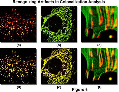
Illustrated in Figure 6 are several of the common artifacts discussed above, which often hamper accurate colocalization analysis in specimens labeled with multiple fluorophores (note that all fluorophore combinations in Figure 6 emit only green and red fluorescence). A human female osteosarcoma epithelial cell (U2OS line) transfected with enhanced yellow fluorescent protein fused to a peroxisomal targeting peptide sequence (green fluorescence), and subsequently immunofluorescently labeled with secondary antibodies conjugated to Alexa Fluor 568 (red fluorescence) targeting peroxisomal membrane protein (PMP-70) is presented in Figures 6(a) and 6(d). The black-level setting for image in Figure 6(a) was too high, resulting in reduced intensity for the yellow fluorescent protein label. This mistake skews colocalization analysis to produce an artificially low detectable level of overlapping pixels from the green channel. The properly leveled image is illustrated in Figure 6(d), which demonstrates a significantly higher degree of colocalization.
The mitochondrial network in a Rhesus monkey kidney epithelial cell (LLC-MK2 line) was co-transfected with enhanced yellow (EYFP) and HcRed1 fluorescent protein vectors containing peptide sequences targeting the mitochondria. During imaging, the much brighter EYFP dramatically overshadows the fluorescence signal from HcRed1, which is almost 100 times weaker when the detector channels have similar voltage, gain, and offset settings (Figure 6(b)). Adjusting the channel values in the HcRed1 detector to equalize the fluorescent protein emission intensities overcomes this discrepancy to reveal a significant amount of colocalization (Figure 6(e)). Note the yellow appearance of fluorescence in the adjusted image compared to the green hues dominating the image captured with closely matched channels.
Mis-registration of overlapping channels is illustrated in Figure 6(c) for a Tahr ovary cell (HJ1.Ov line) stained with Alexa Fluor 488 conjugated to phalloidin (green filamentous actin) and Alexa Fluor 568 secondary antibodies targeting mouse anti-vinculin (focal adhesions). The actin filament ends should colocalize with vinculin in this specimen, but they are slightly out of registration in Figure 6(c), as is a microsphere labeled with red and green fluorophores in the lower right-hand corner of the image. Post acquisition image processing to align the channels (Figure 6(f)) restores the image registration (and that of the microsphere) to produce an excellent candidate for colocalization analysis.
Conclusions
Among the most important points to consider when conducting investigations of fluorophore colocalization is to ensure the highest possible quality of specimen labeling. Antibodies and synthetic fluorophores should be analyzed and chosen for specificity, low background, and lack of cross reactivity. In order to reduce bleed-through artifacts, fluorescent probe combinations with widely separated emission spectra are best suited for colocalization experiments. The proper controls, including specimens labeled with each probe alone as well as an unstained autofluorescence standard, should be prepared and scrutinized for bleed-through under actual experimental conditions. Once the specimen parameters have been optimized, instrument and software considerations can be addressed. It is important to remember that poor specimen preparation usually cannot be overcome by digital image processing techniques. In most cases, perfection of the labeling conditions will save a considerable amount of time and ultimately yield superior results.
Turning to the instrument configuration requirements, the highest quality apochromatic microscope objectives are necessary to reduce the chromatic aberration that will negatively affect quantitative colocalization calculations. Many of the manufacturers have introduced plan apochromat objectives corrected for chromatic aberration over the entire visible light wavelength region (400-700 nanometers), which significantly benefits quantitative fluorescence microscopy investigations. All fluorescence emission filters should be optimized with bandpass transmission characteristics matched to the fluorophore spectral profiles. This is one of the most important considerations for controlling of bleed-through from other fluorophores in the specimen. If bleed-through is detected in controls (single probe and autofluorescence), sequential scanning of the specimen using a microscope equipped with an acousto-optic tunable filter (AOTF) for multitracking will produce the optimum results. In some cases, software correction of bleed-through may be necessary before proceeding with colocalization analysis.