Despite the complex array of settings and adjustments found on modern film cameras and photomicrography exposure control units, exposure of film boils down to a simple relationship between two important variables: the amount of time the film is exposed to light and the intensity of that light. Films are formulated by the manufacturer to respond according to the following formula, E = l × t, where E is the proper exposure, l is the intensity of illuminating light rays, and t is the film emulsion exposure time in seconds or fractions thereof.
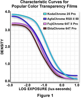
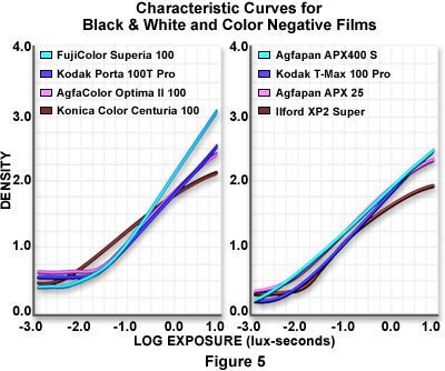
Thus, an increase in light intensity, other things being equal, would call for a shorter exposure time. Similarly, a decrease in light intensity would require a longer exposure time. This linear relationship is known as the reciprocity law and applies to both black & white and color films over a wide range of exposure times and illumination intensities. The response of a film emulsion to exposure and development is often plotted as a graph of film density verses the exposure time (or its base 10 logarithm), and is typically referred to as a characteristic curve. Plotting exposure data by this method was originally suggested by Ferdinand Hurter and Vero Driffeld, and curves of this type have also been termed H and D, Gamma, and D log E curves. Examples of several characteristic curves for popular color transparency films commonly used in photomicrography are illustrated in Figure 1 with a plot of density versus log of the exposure time in lux-seconds. Each film has a unique characteristic curve when processed or developed under a set of standardized conditions. For ease of illustration, the characteristic curves presented in Figure 1 are averaged values for the red, green, and blue emulsion layers, each of which respond in a slightly different manner and display unique values when plotted as density versus log exposure.
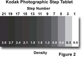
Characteristic curves are obtained by carefully exposing a section of film through a step tablet similar to the one illustrated in Figure 2. After exposure, the film test section is carefully developed under strictly controlled conditions to yield a film strip having a series of steps with sequentially increasing density. Average density of the resulting exposed and processed film is scanned and calculated using an instrument known as a sensitometer. The step tablet produces a series of logarithmic exposure steps on the film, each step differing from the preceding step by a factor of two, or one f-stop. Exposure is described in terms of lux-seconds, which is a measure of the amount of exposure a section of film would receive under a controlled set of conditions. One lux-second is the amount of light received by film placed one meter from a standard candle for a single second.
Film density is a measure of the light-stopping ability of film and is related to the opacity and transmittance of the film. Transmittance is defined as the ratio of light transmitted by the film divided by the total amount of light incident on the film surface. When 50 percent of the incident light is transmitted through the film, the transmittance for that film is equal to 0.5. Opacity is defined as the reciprocal of transmittance, so a film having a transmittance value of 0.5 would have a corresponding opacity of 2.0. Density is defined as the logarithm of opacity, so that a film having an opacity of 2.0 will have a density of 0.3 and, as discussed above, will transmit 50 percent of light incident on the film surface. Film density is dependent upon the quantity of metallic silver present in the developed image.
The shape of a characteristic curve yields a significant amount of information about a particular film and the conditions used to process or develop the film. Several features of a typical characteristic curve (for black & white and color negative films) are illustrated in Figure 3. The curve is generally divided into three distinct regions, a toe region to the left, a linear region in the center, and a shoulder region on the right. Shapes and slopes of characteristic curves vary, depending upon exposure and processing conditions and the film emulsion characteristics.
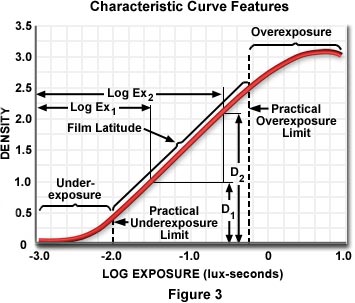
The toe region of the curve is usually crescent-shaped and represents an exposure region where gray tones are compressed, with the separation between shadow densities becoming progressively less when moving from right to left on the curve. The shape and length of the toe region varies from film to film, which is described as being either short-, medium- or long-toed. Short toed films expand shadow tones and are the most useful in low-light level photomicrography. Long-toed films compress tones and are useful in high-contrast situations. The right-hand border of the toe region represents the practical underexposure limit for a particular film.
The linear region of the characteristic curve usually has a constant slope, defined by the following equation (refer to Figure 3):
where Gamma (γ) is historically and traditionally defined as the slope of the linear region, and is useful in scientific and technical photography and photomicrography. Gamma is a measure of the film's contrast and is adjustable through variation in developer chemistry and the amount of development time (and/or temperature). When development time is shortened or low-contrast developers are used to process film, gamma values are decreased. Alternatively, when development time is extended or high-contrast developers are used, the slope of the characteristic curve increases, as does the gamma value. It should be noted that the terms gamma and contrast are not interchangeable.
The linear region of a characteristic curve is also termed the film latitude and represents the useful range of exposure times for a particular film. Color and Black & White negative films display a substantially greater degree of latitude than do color transparency films, primarily because many exposure errors can be corrected during printing. Overexposure is tolerated by negative films much better than underexposure and leads to better prints, although the proper exposure will always produce superior results.
Transparency films produce better results when slightly underexposed, yielding more image detail than when they are overexposed. In general, high contrast films (such as Kodak Technical Pan) or films processed in high contrast developers will have the least exposure latitude, whereas lower contrast films will have the most. The selection of film developer and processing conditions is critical in the final outcome of contrast in negative films. Increased development time usually leads to a decrease in exposure latitude due to an increase in contrast.
Characteristic curves exhibited by transparency films slope in the opposite direction from those obtained with negative films (see Figures 1, 4, and 5). This occurs because a short exposure (underexposure) produces very dense transparencies but thin negatives, and a long exposure (overexposure) yields thin transparencies but dense negatives. In addition, characteristic curves for transparency films have a much steeper slope than negative films, due to the fact that transparency films have more inherent contrast and a very narrow exposure latitude.
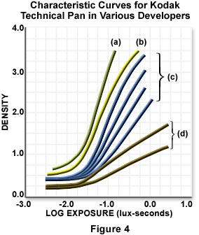
Because each film has a unique response curve, exposure characteristics of individual films can be used to manage image contrast in photomicrography. Specimens inherently lacking in contrast can be photographed with a film having a large characteristic slope to increase contrast in the resulting photomicrograph. Alternatively, with specimens that have too much contrast, a film having a flatter slope can be used to reduce the amount of contrast in the final image. Kodak Technical Pan black & white film displays contrast properties that can be altered over a wide range by proper choice of development conditions, as illustrated in Figure 4. Figure 4(a) shows a response curve for Technical Pan that has been processed in Kodak Versamat 895 developer. The slope of the response curve under these conditions is very steep and images captured on the film will have a great deal of contrast. Successively lower amounts of contrast are produced when other developers are used (Figure 4 (b)-(d). Figure 4(b) illustrates the Technical Pan response curve when Duraflo RT is used as the developing agent, which produces less contrast than Versamat 895 developer. Still lower degrees of contrast are obtained when HC-110 developer is used at varying processing times (Figure 4(c)), and the least amount of contrast exhibited by this film occurs when it is processed with Technidol (Figure 4(d)).
By experimenting with development times and temperatures, a wide latitude of image contrast can be achieved with Technical Pan and other black & white and color negative films. Contrast can also be controlled in color transparency films by adjustment of the first developer process time. When the process time is increased by 15-30 percent, contrast is dramatically enhanced and the film is said to have been push-processed by one-half (15 percent increase) to one f-stop (30 percent increase in development time). Contrast can also be decreased in transparency film by decreasing process time in the first developer. This technique is known as pull-processing, although it is seldom used except in artistic photography.
Every image captured on film is composed of a range of light intensities with highlights positioned on the right side of a characteristic curve and shadows positioned on the left. When a photograph is overexposed, the intensity values all shift towards the right and overall density is increased. Alternatively, when a photograph is underexposed, intensity values shift to the left and resulting film density is decreased.
Exposure Characteristic Curves and Image Contrast
Explore the relationship between the slope (often referred to as gamma) of characteristic curves exhibited by transparency and negative films and the amount of contrast produced by these films.
The shoulder of a characteristic curve is the region where the slope decreases and the curve tends to level off and become horizontal. This region is seldom used in photomicrography because most of the highlights are lost or compressed to such a high degree as to make negatives difficult to print. The start of the shoulder region is the practical overexposure limit of a film.
Careful examination of the characteristic curve for any particular film will reveal critical information about the exposure properties for that film. The central portion of the curve is linear (or approximately so, as discussed above) and is the region where the reciprocity law exposure formula is valid. In this region, 100 arbitrary units of intensity for 1 arbitrary unit of time should result in the same proper exposure as 1 arbitrary unit of intensity for 100 arbitrary units of time. In terms of f-stops and exposure times in traditional photography, an exposure of 1/250 second at f/8 equals an exposure of 1/125 second at f/11. This inverse relationship holds true for most films if the proper exposure duration is between 1/500 of a second and 1/2 second.
However, in microscopy, especially when light altering filters, polarizers, and prisms are added to the optical pathway as in many of the contrast enhancement modes (phase contrast, differential interference contrast, Hoffman modulation contrast, etc.), the proper exposure often is longer than 1/2 second. The film's reciprocity relationship no longer holds, and the film requires additional exposure time to yield proper exposure.
This phenomenon is called reciprocity failure, and it occurs in all color and black & white photographic emulsions regardless of film speed, dye composition, or silver halide concentration. The term "failure" only indicates that the linear relationship between exposure time and light intensity no longer holds and does not indicate a failure of the film emulsion in terms of performance. With classical film characteristic curves, the point of reciprocity failure can be determined by the position and shape of curved regions (the toe and shoulder) occurring to the left and right of the linear portion of the graphs illustrated in Figures 1, 3, 4, and 5. Changes in film response to microscope illumination levels are sometimes referred to as long-exposure effects and short-exposure effects. Under low-light conditions (typical of fluorescence microscopy and polarized light microscopy at high magnifications), exposure times must often be extended to the point of significant film speed loss. Extremely short exposures produce the same effect. Most films also display an increase in scattering of exposed silver halide grains, the formation of smaller latent-image centers, and a lower rate of development at the latent-image centers with exceedingly short exposure times.
The film manufacturers' data sheets and characteristic curves (several of which are illustrated in Figures 1 and 5) suggest how much additional time is needed for proper exposure. Each individual film emulsion has a response tuned to a particular range of illumination values, outside of which the film's response is compromised and the reciprocity law no longer holds. Reciprocity failure can often be compensated simply by an increase in exposure times or processing conditions for black & white films (Table 1), but this is not always the case with color negative and transparency films. Most color films have three color-sensitive dye layers, each of which has a slightly different characteristic curve position and slope resulting in varied responses to the reciprocity effect with the potential to cause undesirable color shifts or casts. Often, both exposure times and color balance filters must be adjusted to compensate for very long or short exposures when using color films.
Adjustments for Long and Short Exposures
Using Black & White Films
| Indicated Exposure Time (Seconds) | Adjusted Exposure Time (Seconds) | Adjusted Developer Time (Percentage) |
|---|---|---|
| 1/1,000 | None | +10% |
| 1/100 | None | None |
| 1/10 | None | None |
| 1 | 2 | -10% |
| 10 | 50 | -20% |
| 100 | 1200 | -30% |
Table 1
Exposure and development adjustments for common black & white films are listed in Table 1. At very fast shutter speeds (1/1000 second and below), these films experience a lowering of contrast or reduced density in the negative, yielding prints that show substantial contrast loss (Figure 6). The only correction for reciprocity failure at fast shutter speeds is to increase the development time, as listed in Table 1. When exposures are very long, typically under low-light conditions, exposure times must be dramatically extended, usually to the point of significant film speed loss.
As mentioned above, very long exposure times are more likely to occur in photomicrography due to low illumination intensity levels that result with contrast enhancing techniques such as fluorescence and polarized light. In fact, exposure times exceeding five minutes are not uncommon, and usually lead to reciprocity failure. When using black & white films, calculated exposure values can lead to negatives lacking shadow detail (Table 1 and Figure 6), but compensation by lengthy exposure often yields too much density in highlight areas, resulting in an increase in overall contrast. This is due to the fact that the reciprocity failure effect is greater in regions where specimen illumination is very low, a problem that can be overcome by increasing the amount of time the film is developed (see Table 1).
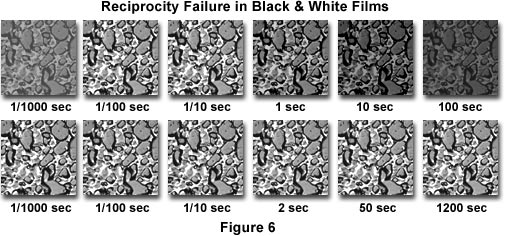
The effect of reciprocity failure in black & white photomicrographs is illustrated in Figure 6, for a series of successive exposures, each increasing by increments of an order of magnitude (1/1000 second to 100 seconds) at constant illumination. The specimen is a thin film preparation of a superconducting ceramic imaged with Kodak Verichrome Pan film and developed for 10 minutes in D-76 developer at 86 degrees (F). Photomicrographs in the upper row of Figure 6 show uncorrected reciprocity failure at the indicated exposure times. Those in the lower row of Figure 6 are corrected with respect to both exposure and development time, as indicated in Table 1.
Exposure Bracketing
In practice, optimum exposure times for any particular film used in microscopy should be determined through experimentation, by conducting a test commonly known as exposure bracketing. Bracketing, the exposure of a series of film frames at varying lengths of time with constant illumination, is typically done using color transparency or negative film, but may be applied to other types of film as well. Start by selecting a specimen having a wide latitude of features including deep shadows and rich highlights, good color saturation, and a significant amount of contrast. Adjust the microscope lamp voltage to the ideal level for photomicrography (usually 8.5 to 9 volts for tungsten-halogen bulbs), ensure the microscope has been aligned for proper Köhler illumination, and place any necessary neutral density, heat shielding, color balancing, and/or color compensating filters into the light path.
Exposure and Color Balance
Explore how exposure settings and color compensating filters can be adjusted to change the contrast, brightness, and color balance of a photomicrograph.
Exposure times should cover the widest range that is practical to guarantee capture of the correct exposure information. With standard SLR camera backs attached to a microscope, it is often necessary to include all exposure times available with the camera shutter. Most backs of this type have shutter speeds ranging from one or two seconds down to 1/500 or 1/1000 second. Holding the illumination voltage constant, focus the specimen and take successive photomicrographs at each shutter speed until the entire range has been covered. Using such a wide range of shutter speeds will ensure the correct exposure time is revealed.
Many modern microscopes are equipped with exposure control systems that meter light using a photodiode or photomultiplier built into the microscope camera system. Often, these control systems have pre-calibrated bracketing capabilities available at the touch of a button. If possible, when using exposure control systems, expose transparency film in 1/3 f-stop increments going two or three f-stops above and below the recommended exposure by the film manufacturer. Exposure latitude for print film (both black & white and color) is much greater than that for transparency films, so bracket intervals of a whole f-stop will be sufficient.
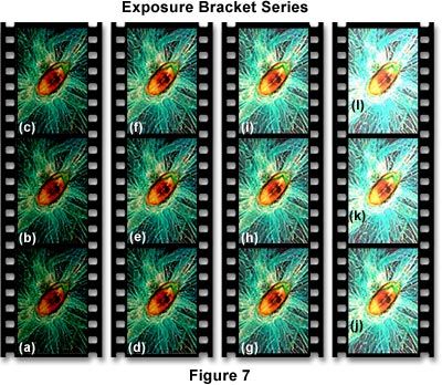
After film containing bracket information has been processed, examine the individual frames on a standard light table with a 5500 K light source (daylight balanced) to determine which frame has the correct exposure. A typical bracket series using Fujichrome 64T transparency film is illustrated in Figure 7. This series was conducted by exposing two f-stops above and below the suggested value with an Olympus PM-30 photomicrography control system. The specimen was a stained silkworm trachea and spiracle imaged in darkfield illumination. The shortest exposure, illustrated in Figure 7(a), is heavily unexposed and very dark. As the exposure time is increased in 1/3 f-stop increments, the resulting frames become progressively lighter (Figures 7(b)-(g)) until the correct exposure is reached (Figure 7(h)). Continuing to increase the exposure time in 1/3 f-stop increments yields still lighter (and overexposed) frames as shown in Figures 7(i)-(l). The exposure time recommended by the PM-30 control monitor was 0.45 seconds (Figure 7(f)), which is almost too dark, or slightly underexposed. Restricting bracket increments to 1/3 of an f-stop allows the microscopist wide latitude in fine-tuning the final film exposure choice. All of the film frames illustrated in the third column of Figure 7 (images (g) - (i)) have acceptable exposures, which lie so close together that a loupe must be carefully used to select the best candidate.
Instead of changing camera shutter speeds or control system exposure times, the microscopist may elect to vary illumination intensity through the use of neutral density filters. It is never a good idea change lamp intensity by varying the voltage supplied to the lamp, because this will seriously affect the illumination color temperature and resulting color response of the film. Always keep the lamp voltage at a constant value and use a series of neutral density filters of increasing transmittance to effect illumination intensity changes. A list of transmittance values and the equivalent exposure increase in f-stops for common neutral density filters is presented in Table 2. Adding a filter of density 0.3 will reduce lamp intensity by a full f-stop (50 percent of the original value - see Table 2). Neutral density filters with a density of 0.1 are also available to decrease the bracket increment to 1/3 f-stop in order to provide a wider exposure range. Filters with a density of 0.15, which increase neutral density by 1/2 f-stop, are also available. Use a combination of filters to cover the entire exposure range. When using neutral density filters to conduct exposure bracketing experiments, adjust the microscope illumination so that a neutral density filter having a density value of 0.6 to 0.9 is positioned in the light path at the start of the experiment. This will guarantee exposures on both sides of the bracket (both over- and underexposed).
Neutral Density Filters in Exposure Bracketing
| Neutral Density Filter | Percent Light Transmitted | Equivalent F-Stop Increase |
|---|---|---|
| 0.1 | 80 | 1/3 |
| 0.2 | 63 | 2/3 |
| 0.3 | 50 | 1 |
| 0.4 | 40 | 1 1/3 |
| 0.5 | 32 | 1 2/3 |
| 0.6 | 25 | 2 |
| 0.9 | 13 | 3 |
| 1.0 | 10 | 3 1/3 |
Table 2
Exposure bracketing can also be conducted using black & white and color negative films. It is often more cost effective to elucidate exposure information with cheaper black & white film, which can be processed in the laboratory. The results can then be translated into comparative exposure values for color negative film. As an example, if a test bracket using Kodak T-Max 200 black & white film indicates a correct exposure at 0.5 seconds, then the same exposure time should work with Fujicolor Superia 200 ISO film. In this case, a one-second exposure could be used when substituting Fujicolor Superia 100 ISO film, a film emulsion with slower response to exposure.
Bracketing is conducted in a different manner when using sheet film. The entire bracket can be performed on a single section of sheet film using either the dark slide of the film holder or the microscope field diaphragm. If the sheet film is held in place using a film holder having a dark slide, first remove the slide and expose the film for a standard unit of time. For instance, if the correct exposure is believed to lie between 2 and 3 seconds, initially expose the entire film section for a single second. Next, push the dark slide into the film holder until it has covered about 1/5 to 1/6 of the film (about an inch), and expose the film again for one second. Push the dark slide in another inch, or 1/5 of the film length, and expose for two seconds. Repeat by pushing in the slide once again and exposing the film for four seconds and so on until the entire sheet has been incrementally exposed. In this manner, the film will have regions exposed in a geometric progression of exposure times (1, 2, 4, 8, seconds etc.), until the entire sheet of film has become an exposure bracket. Process the film and place the sheet on a 5500 K light table. Examine the exposure bracket carefully with a loupe to determine the correct exposure.
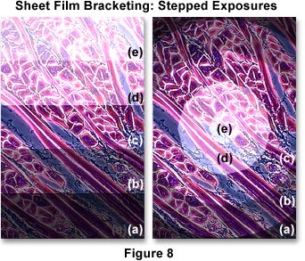
This type of sheet film bracketing is illustrated by the photomicrograph on the left in Figure 8(a) through Figure 8(e). The right hand portion of this figure illustrates a sheet film bracket conducted with the field diaphragm instead of a dark slide. To accomplish this, first expose the entire sheet for a standard unit of time, in a manner similar to that using the dark slide. Then close the field diaphragm until it covers the corners of field of view (and the sheet film) and re-expose for another second. Again, close the field diaphragm another small increment and expose for two seconds. Repeat the procedure until the field diaphragm has been stopped down to the maximum, revealing only a small circular portion of the specimen visible in the central portion of the viewfield. In this manner, a series of concentric circles (Figure 8(a)-(e); right hand side) of varying exposure will be present on the sheet film when it is processed. Choose the correct exposure from the circle that best represents the hues and tonal qualities of the specimen.
Bracketing is a very effective method for determining exposure in optical microscopy, but with such a wide spectrum of magnifications available at varying numerical apertures, it would be an enormous task to bracket film under all possible conditions. This task is not necessary, because once the correct exposure data has been elucidated for a specific set of conditions, exposure times for new conditions can be calculated. It is only when a major change to the microscope optical system is undertaken (such as addition of phase contrast, differential interference contrast, darkfield, etc.) that bracket exposure tests should be repeated. Bracketing is especially useful in fluorescence micrography because of black backgrounds, very long exposures and dangers of fading or permanent bleaching. When translating exposure information from one objective to another, the microscope illumination must be held to a constant value. If a voltage meter is present on the microscope illuminator, always set the lamp voltage potentiometer to the same value for all brackets. If no meter is present, physically place a mark on the microscope body (or illuminator transformer) indicating the correct setting for the voltage potentiometer. This step is very important in order to obtain consistent results in photomicrography.
The primary factors affecting exposure are magnification and the objective numerical aperture. Objectives of different magnifications usually have different numerical apertures, although many objectives having the same magnification can have different numerical apertures depending upon optical correction of the objective. Magnification can also change when new eyepieces are substituted, but this will have no effect on exposure calculations when using microscopes equipped with a trinocular head.
A simple equation has been elucidated by photomicrographer John G. Delly (Photography Through the Microscope) and others to calculate new exposure times in microscopy when the objective magnification and/or numerical aperture has been changed. Exposure varies directly as the square of the magnification and inversely as the square of the numerical aperture. If the optimal exposure time for a particular set of conditions is termed the Standard Time, then a new exposure time can be calculated according to the following equation:
x (New Magnification/Standard Magnification)2
where Standard N.A. is the numerical aperture of the objective used at Standard Magnification in the original exposure bracket tests. New N.A. is the numerical aperture and New Magnification the magnification of the objective having unknown exposure characteristics. The largest variable in using this equation is the manual setting of the substage condenser aperture diaphragm, commonly termed the Working Numerical Aperture as described by the equation:
The opening size of the iris diaphragm should be consistently altered as it is changed from one objective to another. If the condenser has a graduated scale on the periphery, then it is a simple task to set the aperture size each time an objective is changed. Graduated scales are usually presented directly in either condenser numerical aperture, the size of the iris aperture (in millimeters), or in arbitrary units of aperture opening size. When no condenser scale is present, the iris aperture opening diameter at the rear focal plane of the objective must be examined each time to ensure the diaphragm is correctly positioned. A more accurate method to determine the condenser working numerical aperture uses a Bertrand lens and an ocular micrometer. Insert the Bertrand lens into the optical path and use the ocular micrometer to measure the diameter of the diaphragm at the objective rear focal plane with the condenser iris aperture diaphragm both fully opened and reduced to the working size. This data can be used to calculate the working numerical aperture. For example, when an objective having a numerical aperture of 0.50 has a rear focal plane diameter of 14 ocular units and the condenser aperture size is measured at 10 ocular units (OU), the working numerical aperture can be calculated:
Yielding a working numerical aperture (WNA) of:
This degree of accuracy is useful for critical photomicrography with color films at high numerical aperture, but is often not necessary for routine photomicrography. As an alternative, the microscopist can simply place marks beneath the diaphragm adjustment lever (on microscopes so equipped) to indicate the approximate correct settings.
In practice, the exposure calculation equation is quite simple to use. Suppose that the standard time for a 25x objective of numerical aperture 0.40 is 0.15 seconds. To calculate the new exposure time for a 10x objective having a numerical aperture of 0.25, use the following numbers:
New Exposure Time = 0.15 × 2.56 × 0.16 = 0.06 seconds
Thus, the new exposure time for the 10x objective is 0.06 seconds, a little less than one half the standard exposure time. It is quite convenient to construct a table of exposure times using the various objectives available for each film that is being used. A good alternative to this practice is to use our interactive Flash tutorial to calculate exposure times.
Exposure Calculation in Photomicrography
Use a known film exposure time measured from brackets under standardized conditions of magnification and numerical aperture to determine exposure for a new objective of different magnification and numerical aperture.
The equations described above are useful in computing exposure time when using standard dry objectives and condensers in optical microscopy with common specimens. However, when the objective and condenser form part of a complete oil immersion system, the loss of light by reflection is greatly reduced and film exposures may be decreased by as much as one-half. We recommend separate determination of exposure brackets for dry and oil immersion objectives.
In reflected light systems where the field is illuminated through the objective (using a vertical illuminator), the exposure calculation equations also fail, because exposure varies little with a change of objective at the same magnification. Other factors, such as the nature of the specimen, also play a critical role in exposure calculation and should be kept in mind when determining film exposure parameters.
Changing to a film of new ISO rating also changes the exposure time. A simple equation can be applied to calculate the new film exposure time when changing film speed:
Where Standard ISO is the film speed (or ASA) of the film having known exposure parameters, and New ISO is the film speed (or ASA) of the new film. As an example, if the correct exposure time for a specimen using Fujichrome Velvia (ISO = 50) is 0.2 seconds, the adjusted exposure time when Fujichrome Provia (ISO = 100) is substituted can be calculated:
New Exposure Time = 0.1 seconds
Both of the equations described above are very useful in calculating exposure time for photomicrography under a set of standardized conditions. In fact, these two equations can be combined to form one universal equation for a majority of exposure calculations:
where Std Time is the experimentally determined exposure time at standard numercial aperture (Std N.A.), magnification (Std Mag.), and ISO (Std ISO). The calculated exposure time (New Exposure Time) is determined by the new numerical aperture (New N.A.), magnification (New Mag.), and new ISO (New ISO). This calculation is conveniently performed by our interactive Flash tutorial:
Exposure Calculation (With ISO Correction) in Photomicrography
Use a known film exposure time measured from brackets under standardized conditions of ISO, magnification, and numerical aperture to determine exposure for a new objective of different magnification and numerical aperture using a film with a new ISO value.
It is very important to adhere to a strict set of parameters when determining baseline standards for exposure brackets using the most common objectives. When this is accomplished, new objectives and films can be used to the greatest effect without serious miscalculations in exposure, which usually results in unsatisfactory photomicrographs.
Filter Factors
When colored filters are introduced into the microscope light pathway, a portion of the white light color spectrum is restricted by the filter, reducing illumination intensity and increasing exposure time. The amount of light absorbed by a filter is determined by the wavelength spectrum passed by the filter, which varies from most of the visible light spectrum being passed to cutoff filters approaching monochromatic illumination. Exposure increases with colored filters are also dependent upon the spectral sensitivity of the film being used. It is common to use specific light filters in black & white photomicrography to control contrast in stained specimens. Use of colored filters necessitates a careful determination of exposure to ensure properly exposed photomicrographs having good tonal balance and contrast.
After exposure parameters have been determined under a set of controlled conditions using white light from the microscope lamp (no filters present), a new set of parameters must be introduced to compensate exposure times when a filter is added. The amount of change in exposure time is commonly termed a filter factor, and almost always represents an increase in exposure time. Filter factors are often published in literature accompanying the film, or they can be determined experimentally (the best choice). The exposure time measured or calculated without a filter can be multiplied by the filter factor to determine the amount of exposure adjustment necessary when the filter is in place. When using an exposure meter to measure illumination intensity, remove all filters to avoid a non-uniform response by the photocell, which may not be equally sensitive to all wavelengths of the visible light spectrum. In practice, the best approach is to measure exposure times in white light, then apply either measured or calculated filter factors to determine exposures.
Published filter factors should only be considered as a good approximation, because these factors can vary with the spectral response of photographic materials and the color temperature of the light source. Exact filter factors are best determined experimentally using a controlled set of conditions. To establish a baseline for filter factor exposure calculations, first conduct exposure brackets using white light without any filters in place. Next, repeat the experiment with the desired filter or filter combinations in the optical pathway. For these experiments, especially when using brightfield illumination, it is not always necessary or preferred to have a specimen in place on the microscope stage. Equally good data can usually be obtained from the background light intensity alone. Exposures should be conducted in a geometrical progression (for example exposures of 1, 2, 4, 8, 16, 32 seconds and so on) using a constant voltage setting on the microscope lamp.
Filter Factors for Kodak Technical Pan Film
| Kodak Wratten Filter Number | Tungsten Filter Factor | Daylight Filter Factor |
|---|---|---|
| No. 8 (Yellow) | 1.2 | 1.5 |
| No. 11 (Yellowish Green) | 5 | --- |
| No. 12 (Deep Yellow) | 1.2 | --- |
| No. 15 (Deep Yellow) | 1.2 | 2 |
| No. 25 (Red) | 2 | 3 |
| No. 47 (Blue) | 25 | 12 |
| No. 58 (Green) | 12 | --- |
Table 3
After establishing exposure brackets (or stepped exposures) with and without the filter(s), the brackets can be compared to determine which steps match in density. For example, if a one-second exposure in white light produces a photomicrograph of a particular density and a 4-second exposure with the selected filter produces the same density, then the exposure (filter) factor for that filter is 4. When using a different specimen with the same filter, multiply the exposure of the specimen in white light by a factor of 4 to obtain the correct exposure. Table 3 presents a listing of filter factors suggested for Kodak Technical Pan black & white film, which is typical for films of this type.
The best photomicrographs present an image of the specimen with sharp and crisp details, good exposure in both highlights and shadowed areas, and excellent color saturation. Determination of the correct exposure in photomicrography is much easier when transparency films are being judged. These films have a very narrow exposure latitude, usually one-half to one f-stop, and incorrect exposure is very obvious. With transparency film, a good exposure will reveal specimen details in all areas of the photomicrograph, unless this detail is actually missing in the specimen. Transparency film that has been overexposed will have a thin appearance with washed-out highlights lacking in detail. When transparency film is underexposed, shadowed areas tend to go black with a total loss of detail. The overall appearance of the film will be very dark. As a general rule of thumb, correctly exposed transparencies will have observable density in the brightest highlight regions.
Exposure with black & white and negative films is much harder to judge. These films exhibit a far greater exposure latitude than that found with transparency films, but examination of the results usually occurs at the film negative stage. Negative films will tolerate overexposure to a far greater degree than underexposure. Light areas on the negative translate into dark areas on the final print, and it is these regions that should be used to judge overall quality of the photomicrograph. If the film is overexposed, little detail will be present in light areas on the negative, and these areas, which translate into dark areas on the print, will likewise be devoid of detail when printed. When correctly exposed, negative films will reveal details in both light and dark regions of the negative, which translate into prints with good specimen rendition in highlights, background, and shadowed areas.