Depending upon the illumination conditions, specimen integrity, and preparation methods, digital images captured in the optical microscope may require a considerable amount of rehabilitation to achieve a balance between scientific accuracy, cosmetic equilibrium, and aesthetic composition. When first acquired by a charge-coupled device (CCD) or complementary metal oxide semiconductor (CMOS) image sensor, digital images from the microscope often suffer from poor signal-to-noise characteristics, uneven illumination, focused or defocused dirt and debris, glare, color shifts, and a host of other ailments that degrade overall image quality.
After an image has been acquired from the microscope, it is commonly referred to as a raw image and should be catalogued and saved before commencement of image processing or analysis operations. This step will ensure that an original copy of the image is available in case irreversible mistakes are made during image processing or the image is lost or otherwise rendered unrecoverable. In addition to the raw image, a background image or flat-field frame should also be recorded with the specimen removed from the optical path to generate an image of the background without the specimen. The best method is to relocate the viewfield to an area of the slide that contains mounting medium and the coverslip, but does not have a significant level of debris, in order to simulate the background illumination profile. An alternative method is to defocus the microscope with the specimen in place, and then record a background image. Although the latter technique is not preferred, it is sometimes the only alternative, particularly if the specimen occupies a majority of the area underneath the coverslip. In situations where quantitative information must be derived from the specimen, several background images can be averaged together to reduce the level of noise.
In addition to a background image, it is often wise to also record a dark frame to establish the dark (electronic and thermal) noise level of the digital camera system. The dark frame should use the same exposure as the original raw image, but is obtained without opening the camera shutter. In some cases, it may be necessary to detach the camera from the microscope and cover the mounting adapter with a lens cap or a section of black cardboard. As with the flat-field frame or background image, multiple dark frames can be collected and averaged together. After all of the necessary images have been gathered (raw, background, and dark), image processing operations can proceed.
Background Subtraction
Examine how a background subtraction image can be created from a raw digital image captured in the microscope with this interactive tutorial. Background regions used in the calculations can be selected with control points to generate a wide spectrum of possibilities.
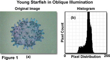
A typical image captured in oblique illumination with an optical microscope coupled to a digital camera system is presented in Figure 1(a). The specimen is a fixed and stained young starfish (just after metamorphosis) prepared as a whole mount in imbedding medium, and sandwiched between a glass slide and coverslip. Because of uneven illumination problems frequently encountered with off-axis lighting techniques, this specimen was chosen to illustrate problems that are emphasized due to the large visible background region. Oblique light from the microscope illuminator produces a somewhat uneven background (often appearing as a gradient of intensity), as is evidenced by the brightness variation in Figure 1(a). There is, in addition, a greenish cast to the entire image that is caused by incorrect white balance adjustment of the CCD image sensor. Furthermore, the image was captured at a relatively low light level, which increases the amount of random noise present in the image (note the grainy appearance of the background and specimen).
A gray-level image histogram (Figure 1) of the original raw image reveals that only a small portion of the CCD image sensor's dynamic range was utilized in producing the image. A vast majority of the gray levels in the image are clustered in a region between values of 60 and 210 with very few pixels exhibiting levels that are either higher or lower. This restriction of the histogram gray-level values to the center of the scale produces poor image contrast (see Figure 1(a)) that must be corrected during image processing. The large spike in gray levels centered on 140 corresponds to the intensity level representing the background color. As the background becomes more uniform (reducing the number of gray levels) during processing, the width of this distribution will narrow, and the pixel count will increase.
Image processing of the optical micrograph illustrated in Figure 1 can be accomplished with a number of commercially available software packages. Recommended low-cost aftermarket image-editing software includes Adobe Photoshop, Corel Photo-Paint, Macromedia Fireworks, and Paint Shop Pro. In addition, higher-end software programs, designed specifically for digital images from the microscope, can be utilized to perform the necessary image-editing functions. Many of these programs incorporate algorithms that simplify commonly utilized steps in optical micrograph image processing, such as background subtraction, flat-field correction, histogram manipulation, and gamma correction.
Brightness and Contrast in Digital Images
Explore the wide range of adjustment that is possible in digital image brightness and contrast manipulation, and how these variations affect the final appearance of both the histogram and the image.
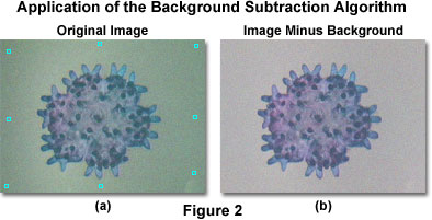
The first step in image processing is to remove brightness fluctuations (due to uneven background illumination) and noise introduced by the specimen or camera system. For a majority of digital images, simple background subtraction algorithms are sufficient and will produce corrected images that have even brightness values across the image. However, with images destined for quantitative analysis requiring photometric accuracy, flat-field correction is the preferred technique.
The raw starfish image illustrated in Figure 1(a) was adjusted with a background subtraction algorithm (Figure 2(a)) to produce the corrected image presented in Figure 2(b). The algorithm employs user-selectable control points that can be strategically relocated around the image to specify brightness values within selected regions of the background. After placement of the control points, their representative brightness values are utilized to fit a surface function for creation of an artificial background. The calculated background is then subtracted from the specimen image to obtain a least squares fit of the surface function that approximates how the background would appear with even illumination. In practice, the control points should be chosen so that they are evenly distributed across the image (as they are in Figure 2(a)), and the brightness level at each control point should be representative of the overall background intensity.
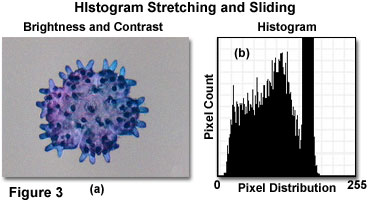
After background subtraction or flat-field correction adjustments have been applied to the image, the next step is to restore brightness and contrast levels to match the appearance of the specimen in the microscope (either through the eyepieces or on the live video feed to the camera interface software). Histogram stretching and sliding operations typically appear as brightness and contrast adjustment sliders in the common image-editing software programs. More sophisticated manipulation of the histogram profile is usually possible in high-end software packages, but the basic tools available in all image editors can often be utilized to perform satisfactory adjustments to the image.
The starfish specimen image, after being corrected for background subtraction, contrast deficiencies, and brightness variations, is illustrated in Figure 3(a). Note how the stained appendages have become more clearly defined and the overall image contrast has improved. In addition, the background has been shifted from a greenish fluctuating gradient to a smooth (when overlooking the grainy noise) and even gray tone. The modified histogram is presented in Figure 3(b), and can be compared to the original raw image histogram in Figure 1(b). After processing, the histogram is stretched to cover a wider range of gray levels (10 to 220 versus 60 to 210) with additional pixels shifted to darker values. As a result, shadow tones in the corrected image appear deeper and richer than in the original, and the contrast level is much higher.
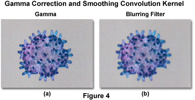
The next step in processing is adjustment of gamma to enable exponential scaling for the purpose of simultaneously displaying both bright and dark features of the image on a computer monitor. Presented in Figure 4(a) is the starfish specimen image after gamma correction. When adjusting a computer monitor that will be utilized for image processing, the gamma correction depends, in part, on the brightness and contrast control settings on the monitor. The monitor controls enable the microscopist or digital artist to alter gamma correction to suit individual tastes and compensate for variability between presentation formats, such as individual web browsers on a variety of computer operating system platforms.
Gamma Correction
Discover how intensity distribution and the relationship between contrast in dark and light regions of a specimen can be adjusted with gamma correction algorithms.
In order to reduce or eliminate random noise from the image, a specialized convolution kernel, known as a smoothing filter is often applied to the image. In most image-editing software programs, this type of operation is referred to as a noise (often specifically designated for dust and scratches), blur, or Gaussian blur filter. Some of the algorithms have user-configurable controls, while others simply apply a series of fixed settings to the image. Proper application of smoothing filters can effectively remove noise, scratches, and other high-spatial-frequency artifacts from digital images. Noise in the starfish specimen image (readily apparent in the background) has been removed by filtration in Figure 4(b) to produce a smooth background, but noticeably softer (more blurred) image features.
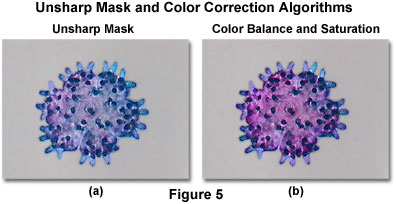
Once the noise and other imperfections have been removed from the image, a sharpening algorithm can be applied to remove some of the low-frequency spatial information and enhance the definition of fine edge detail. Many of the popular image-editing programs contain an unsharp mask algorithm that is ideal for this purpose. One of the primary advantages of the unsharp mask filter over other sharpening filters is the flexibility of control, because a majority of the other filters do not provide any user-adjustable parameters. Illustrated in Figure 5(a) is the starfish specimen after an unsharp mask filter has been applied to increase edge detail. When compared to Figure 4(b), which is the same image after application of a Gaussian blur filter, the dramatic enhancement of fine detail is obvious. Care should be taken not to over-apply sharpening filters, which can re-introduce noise and similar artifacts into the image and, when taken to an extreme, produce severe pixelation at the edges.
Adjustment of Digital Image Sharpness
Discover how sharpening an image using the common unsharp mask filter algorithm can altering the definition and contrast of features and image details.
The final step in processing is to correct the color balance and adjust saturation of the image to remove unwanted color casts and return image colors to those observed in the microscope. Most image-editing software programs contain a settings panel that enables the operator to adjust hue, saturation, and color balance of images captured with the microscope. The color correcting algorithms are applied through the use of sliders (or text input boxes) to either increase or decrease saturation, or transition through various hues and color balance ratios.
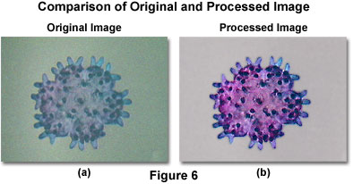
After the image processing steps have been completed, the adjusted image can be compared to the original raw image (see Figures 6(a) and 6(b)) to determine how much improvement has been achieved. It is evident, by examining Figure 6, that overall image contrast, brightness, and saturation is remarkably better in the processed image. In addition, the uneven background has been replaced by a nearly-uniformly gray matte substitute, with elimination of the green cast. Noise has also been reduced, and the fine image details are noticeably sharper.
Balancing Color in Digital Images
Observe how color balance, hue, and saturation can be manipulated to eliminate unwanted casts and restore the original colors to a digital image. This tutorial contains interactive controls that enable the visitor to adjust a wide spectrum of color variables in selected images.
As discussed above, the processing steps can be accomplished with popular image-editing software or through the interface included in software packages accompanying many digital camera systems. Although the some of the camera software programs contain basic image processing algorithms that perform adequately, many of the more complex programs designed specifically for image-editing contain additional features that can be utilized to create special effects or conduct measurements at any stage of the processing scheme. For example, Adobe Photoshop contains a wide range of filter algorithms, which enable the operator to apply stylizing features, de-speckle or distort the image, and add special effects such as brush textures and lens flare. In fact, this program is so comprehensive that images captured with the microscope can be rendered into completely different manifestations, which bear little resemblance to the original raw image. If the purpose of image processing is to rehabilitate and restore the image for scientific measurement or presentation, then use of auxiliary image-editing algorithms should be kept to a minimum and applied only when necessary. However, if the image is destined to be modified for artistic purposes, then the wide spectrum of special effects available in modern software programs can be applied without regard to scientific accuracy.