Understanding the Link Between Digital Image Data and Biological Samples
This white paper explores the link between the signals in biological samples and the digital data from microscope cameras. Understanding this relationship can help you set the ideal image acquisition conditions to achieve the highest quality images and data.
The Fundamentals of Digital Imaging
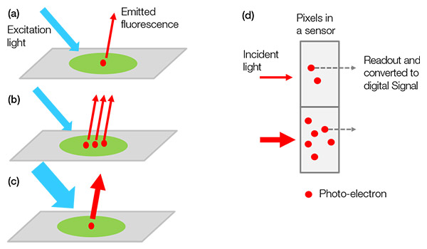
A microscope monochrome camera is a device that detects and visualizes the light from biological samples. The microscope observes the fluorescence light emitted from fluorescence dyes or proteins, then the camera detects this light and converts it into photoelectrons to be detected as a digital signal.
The detected signal value is a complex multiplier of the number of labeled targets (e.g. targeted proteins), excitation light intensity, and efficiencies of excitation and fluorescence emission/detection, including the camera’s conversion efficiency from light to digital signal (Figure 1).
When you use the same system and image acquisition settings for different samples in one experiment, all components except for the amount of the target become constant values, making the detected signal value proportional to the amount of the target. This means, for example, that you could quantitatively compare a gene-edited sample with its wild type.
Figure 1 – From sample to digital signal: (a) an excited labeled target emits fluorescence light. |
The Anatomy of Signal and Background Noise
This section explains the core factors that contribute to image quality and highlights the importance of carefully taking images during an experiment.
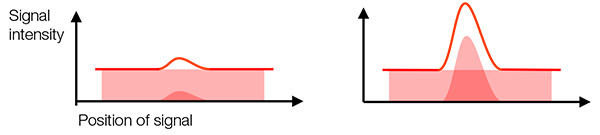
Actual signal vs. background signal: The detected signal contains actual signal and background signal (background noise). To detect your target by identifying it from background signals, you need a high enough ratio of actual signal intensity vs. background signal (Figure 2). This is called the signal-to-noise ratio (SNR). Aiming for a higher SNR leads to better image quality and quantitative analyses.
In general, maximizing the actual signal (e.g. with a higher NA objective) and minimizing the background signals (e.g. with a darkroom, deeper cooling, or a high quantum efficiency camera) are common ways to improve the SNR.
Please note that the gain setting, which defines the amplification factor in a camera for signals, does not improve the SNR because it impacts both actual signal and background signal.
Figure 2 – Left: low SNR: background noise makes it difficult to identify the actual signal. |
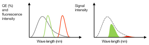
Actual signal: As we mentioned before, using a high NA objective can help improve the SNR. Another important factor to obtain a stronger signal is a high quantum efficiency (QE). The QE indicates the conversion efficiency from incident light to photoelectron. Keep in mind that a camera cannot sense light if its QE is zero percent at a certain wavelength. For example, we must choose a camera with a sensitivity over 720 nm to use near infrared (NIR) dyes like Cy7 for an NIR window in biological tissues or for preventing crosstalk while multiplexing.
Figure 3 – Left: the gray line is the QE of a camera. Green and red lines indicate fluorescence emission spectrum. Right: the detected signal value is equal to the area size, which is a multiplier of the QE and fluorescence spectrums in the left figure. In this case, even if the fluorescence light has enough intensity, the detected signal could be weak for red fluorescence due to low QE. |
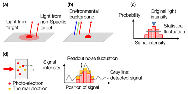
Background noise: Background signals can be categorized as:
a) biological background signals
b) non-biological background signals
c) statistical fluctuation of a photoelectron (shot noise)
d) noises in a camera
The shot noise is unique and can be compared to a coin toss. Just like a 50% probability of showing “heads” might lead to “tails” on two coin flips, any trial with the number N has a statistical fluctuation of ±√(N). The detected number of photoelectrons follows the same rule.
All the background noise examples are shown in Figure 4 below.
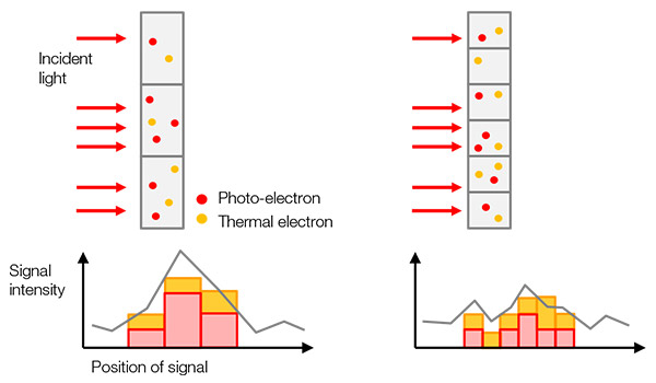
Figure 4 – Examples of background noises: (a) biological background from a non-specific stain or autofluorescence, (b) environment light from the room reflected on a slide, (c) shot noise, (d) noises in a camera that contain thermal electrons generated in a sensor (left) and readout noise (right). Thermal electrons can be reduced by cooling the sensor. |
Resolution: A larger pixel size or binning image acquisition can capture more light and provide a higher SNR, but the larger pixel size lowers the resolution (Figure 5). Consider the best pixel size that aligns with the optical resolution.
Figure 5 – Left: a larger pixel size provides a higher sensitivity but lower resolution. |
Best Practices for Using Microscope Cameras
Although the ideal image acquisition settings vary depending on the application and sample, two common parameters are excitation light intensity and exposure time. Longer exposure time or stronger excitation light provide brighter fluorescence, leading to a higher SNR. However, this also worsens phototoxicity. This brings up an important question: how do you set the best image acquisition parameter to achieve longer live cell imaging experiments while reducing damage to the cells caused by excitation light.
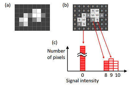
To determine the ideal exposure time, use an image histogram. The X axis of the histogram is signal intensity. The height of the histogram at each X value shows the number of pixels for the signal intensity (Figure 6).
Figure 6 – A histogram of an image. (a) Original image, (b) signal intensity of each pixel shown in the original image, |
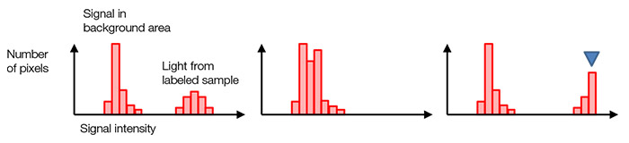
Usually the black background pixels have a non-zero digital signal value even with no background light (Figure 7, left). This helps to avoid a negative value signal caused by the readout noise fluctuation mentioned in Figure 4 (d). The shape and distribution of the histogram tell us if the current exposure time is appropriate. If the histogram is too crowded in a low signal range, then the exposure time is too short (Figure 7, middle). If there is a sharp cliff at the maximum signal level, then the signal value is saturated (Figure 7, right). In this case, you can reduce the excitation intensity or shorten the exposure time.
Figure 7 – A histogram at normal exposure (left), under exposure (middle), |
Some image acquisition software have an automated display adjustment feature that provides better visibility while maintaining the original image data. In most cases, a monochrome camera’s signal dynamic range (e.g. 16-bit = 65,536 levels) is wider than a display’s dynamic range, which is usually 8-bit (= 256 levels).
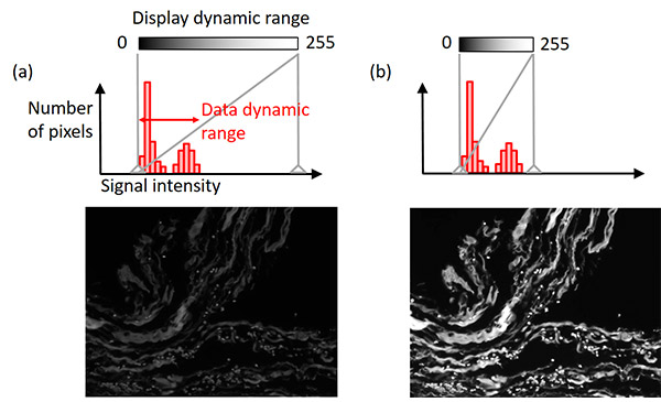
The display adjustment feature defines the link between signal intensity and the display brightness. Usually the intensity from the brightest signal in your sample is much lower than the maximum intensity the camera can handle. In this case, matching the display dynamic range to the data dynamic range (the range from background level to the brightest signal) enables you to get better visibility while maintaining the original image data (Figure 8). A histogram helps to illustrate this adjustment.
Figure 8 – Display adjustment: (top) a histogram with the display setting indicator in a gray solid vertical line, (bottom) the example image. Left example image: original display setting. Right example image: display condition adjusted while maintaining the original image data. |
6 Steps to Set Up a Microscope Camera’s Acquisition Parameters
To summarize, here are six general steps to properly set up a microscope camera for an experiment. Please note that the best procedure depends on your specific application and samples.
- Determine the observation magnification.
- Adjust the focus on your sample, and find the observation target. Consider using a higher gain or binning mode on the camera to shorten the process and minimize phototoxicity. We also recommend that you use an automated or manual display adjustment to observe the signal under its best condition and close the excitation light shutter whenever you’re not observing the image.
- Set the gain and binning mode back for image acquisition.
- Try the gentlest excitation light intensity, and check if you can observe the signal in a realistic exposure time. If you cannot identify the signal, or if the SNR is too low, try a longer exposure time.
- If the exposure time is unrealistically long or longer than the maximum exposure time allowed for the image acquisition speed, try a slightly higher excitation intensity step by step.
- Check the histogram to confirm there is no saturation.
Conclusion
While many complex factors contribute to image and data quality in the microscopy process, knowing these digital imaging basics and tips can help you determine the best acquisition setting for each experiment. Maximizing the signal, minimizing the background, and optimizing the sample condition are essential elements to improve data quality for any application and experiment.
Author
 |
Takeo Ogama
Scientific Solutions Division OLYMPUS CORPORATION OF THE AMERICAS |
Sorry, this page is not
available in your country.