Resolution in optical microscopy is often assessed by means of an optical unit termed the Rayleigh criterion, which was originally formulated for determining the resolution of two-dimensional telescope images, but has since spread into many other arenas in optics.
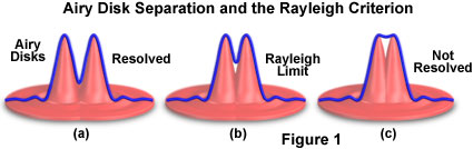
The Rayleigh criterion is defined in terms of the minimum resolvable distance between two point sources of light generated from a specimen and is not dependent upon the magnification used to produce the image. In a two-dimensional image, two point sources are resolvable if their Airy disk diffraction patterns are distinct. According to the Rayleigh criterion, two closely spaced Airy disks are distinct if they are farther apart than the distance at which the principal maximum of one Airy disk coincides with the first minimum of the second Airy disk (as illustrated in Figure 1). If the point sources are of equal wavelength, then their Airy disks have the same diameter, and the Rayleigh criterion is then equal to the radius of one Airy disk, measured from its point of maximum intensity to the first ring of minimum intensity. For monochromatic images of a given fluorescence wavelength, the Rayleigh criterion can be estimated using a standard formula that is found in many optics and microscopy textbooks:
where d is the Rayleigh criterion, λ is the wavelength of emitted light, and NA is the objective numerical aperture. Note that the smaller the value of d, the higher the resolution.
Illustrated in Figure 1 are mathematically generated light intensity profiles (blue line) from two point sources of light. The profiles can be considered to represent pixel intensities along a line through the Airy disk (in effect, the x-y image of the point spread function at focus). The Rayleigh criterion for resolution is met when the maximum intensity of one point spread function overlaps the first minimum of the other. For two points emitting at the same wavelength, this separation distance corresponds to the radius (or peak-to-minimum distance) of the central bright region of a single point spread function.
The resolution formula outlined above is useful for assessing resolution in the image plane, but not along the optical axis (z-axis) of the microscope, information that is critical to successful analysis by the deconvolution technique. However, an adequate formula for the axial Rayleigh criterion can be deduced using similar reasoning. The minimum resolvable axial distance between two point sources of light will occur when their axial diffraction patterns are distinct. This is complicated by the fact that the axial diffraction pattern of a point source is not disk-shaped, but has the hourglass shape or flare of the point spread function image in the x-z or y-z planes. Nevertheless, this hourglass shape has a central bright region, as does the Airy disk. Therefore, the axial Rayleigh criterion can be defined by taking the distance from the point of maximum intensity to the first point of minimum intensity of the central bright region along the z-axis. This value can be estimated using the following formula:
Note that the formula includes η, the refractive index of the mounting/immersion media, in the numerator. The mounting and immersion media are assumed to have the same refractive index; otherwise, spherical aberration leads to degradation of resolution. The reader should also note that all of the criteria discussed assume aberration-free imaging conditions, an unrealistic scenario in practice. Careful scrutiny of the axial resolution equation listed above indicates that reducing the refractive index of the immersion medium can improve z-axis resolution. However, this does not occur because the objective numerical aperture (also dependent upon the refractive index value) is reduced when an imaging medium having lower refractive index is introduced. Because axial resolution varies with the square of the numerical aperture, the reduction in objective numerical aperture outweighs the gain achieved by reducing the refractive index of the imaging medium, and resolution is compromised. Notice also that resolution in the x-y plane varies only with the first power of numerical aperture, whereas axial (or z-axis) resolution varies with the square of the numerical aperture. This important difference means that x-y resolution and z-axis resolution both improve with increasing numerical aperture, but z-axis resolution improves more dramatically.
Z-resolution is closely related but not identical to the concept of depth of field. The depth of field is classically defined as the thickness region of the specimen that appears in focus in the final image at a particular focal setting of the microscope. When examining a two-dimensional image, a certain portion of the specimen is focused onto a single plane. Features that appear equally well in focus in the image may reside at different depths in the specimen. The definition of focus is somewhat subjective, but a standard depth of field "unit" is often defined as half the axial Rayleigh unit:
Another criterion that is occasionally utilized instead of the axial Rayleigh criterion is the full width at half maximum (FWHM) of the central bright region of the point spread function. Formulas for estimating the full width at half maximum in confocal microscopy appear in several microscopy reviews and are identical to those described above for the Rayleigh criterion in widefield microscopy. It should be emphasized that these are rough expressions that give practical estimations. They are not exacting analytical formulas, which would require vector wave theory.
It should also be understood that any resolution criterion is not an absolute indicator of resolution, but rather an arbitrary criterion that is useful for comparing different imaging conditions. The Rayleigh criterion applies specifically to the case in which two self-luminous objects must be distinguished. In other contexts, such as differential interference contrast (DIC), brightfield, or darkfield microscopy, other criteria will apply. In some applications, such as localization of a moving object, resolution below the Rayleigh limit is possible. This highlights the fact that resolution is task-dependent and cannot be defined arbitrarily for all situations.
In addition, resolution also depends to a great extent on image contrast, or the ability to distinguish specimen-generated signals from the background. Contrast depends largely on specimen preparation techniques such as fixation quality, antibody penetration, evenness of staining, fluorophore fading, and background fluorescence. Optimizing specimen preparation methodology can improve resolution more dramatically and at a lower cost than optics or computers. However, assuming a high-quality preparation, the limit of resolution for any application is always dependent on the point spread function, and the Rayleigh criterion yields at least a basic handle on the magnitude of this value.
Resolution and Contrast Improvement
Within the framework of principles upon which deconvolution algorithms are based, it is reasonable to question what degree of quantitative improvement in image quality can be expected from iterative deconvolution, and how best to evaluate and compare the performance of various algorithms. One means of making such an assessment is to measure the size and brightness, before and after deconvolution, of a test object of known size. Figure 2 presents data from image stacks of a subresolution (0.1 micrometer) fluorescent bead acquired with a widefield imaging system utilizing an oil immersion objective (1.4 numerical aperture). All aberrations were carefully minimized before data collection, and because there is no out-of-focus signal from any other object, the minute bead represents a nearly ideal specimen for this purpose.
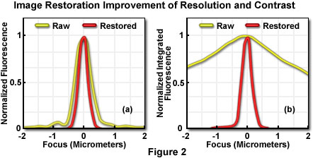
In Figure 2, the yellow lines represent raw image data, while the red lines illustrate data from images restored by constrained iterative deconvolution. For purposes of scaling on the graphs, each intensity value has been normalized to the maximum value of its own image stack. Without such normalization, data from the raw image would barely be visible on the graph because pixel intensities near focus are so much brighter in the restored image than in the raw image. The total integrated intensity of each image stack, however, is the same in both cases.
To quantify the improvement in resolution achieved by iterative deconvolution, pixel intensities were measured on a line parallel to the optical axis through the center of the bead, before and after restoration. Each pixel's intensity was plotted (Figure 2(a)), after normalization, as a function of distance along the z-axis from the center of the bead (0 micrometer). The full width at half maximum (FWHM) of the z-axis intensity profile is taken as the bead diameter, and measures 0.7 micrometer in the raw image and 0.45 micrometer in the restored image (the actual object measures 0.1 micrometer). This modest increase in resolution due to the restoration would only rarely reveal a biological specimen structure that was not visible in the raw image.
A major change in the image resulting from the restoration is apparent in the data presented in Figure 2(b), which represents the sum of all pixel values in each focal plane (the integrated pixel intensity) as a function of focal depth. The curve corresponding to the raw data (before processing) shows significant out-of-focus intensity at 2 micrometers distance from the bead. Restoration by iterative deconvolution shifts the majority of the out-of-focus intensity back to its focal plane of origin. The result is a significant improvement in image contrast, making it easier to resolve and distinguish features in the image. In plotting this data, the summed intensities of pixels in each focal plane of the raw and restored image stacks were normalized to the minimum and maximum values of the plane's image stack. Summed intensity is plotted as a function of focal (z-axis) distance from the bead center (0 micrometer). The restoration of signal intensity from out-of-focus specimen volume to in-focus produces a major contrast improvement, as well as an increase in signal-to-noise ratio. It should be noted, however, that the integrated intensity of the entire image (in effect, the sum of the summed intensities of each plane) is the same in the raw and restored images.
The previous discussion outlines one means of evaluating the performance of an iterative deconvolution algorithm. Determination of which algorithm, of the many available, produces the best restoration presents another problem to the microscopist. A number of Web sites compare the results of applying different algorithms, but such comparisons can be misleading for a variety of reasons. First, algorithms are often compared by implementing them to restore images of synthetic spherical objects, such as the bead employed to collect the data presented in Figure 2, or even computer-generated images of theoretical objects. The relationship between performance evaluated utilizing test objects and performance with actual biological specimens is not straightforward. Furthermore, unless the comparison is done quantitatively, with objects of known size, it is difficult to assess whether a more pleasing result is really more accurate. For instance, the algorithm might erode the edges of features, making them appear sharper, but confounding measurements.
An additional problem is that algorithm comparisons are usually published by parties with an interest (often financial) in the result of the comparison, which makes them potentially biased. Commonly, these parties compare a deconvolution algorithm whose implementation they have developed and refined over many years, with a non-optimized algorithm that is implemented in its most fundamental form, as originally published. However, as discussed previously, large differences in speed, stability, and resolution improvement can be attributed to details of the implementation and optimization of an algorithm. Therefore, the only fair comparison is between realized software packages, rather than between basic algorithms.
It is strongly recommended that any potential buyer of deconvolution software compare the performance of various software packages on their own data. This may require a degree of determination because many companies' sales representatives will routinely save images in a proprietary file format, which often cannot be opened by competitors' software. To compare images restored by different software packages, it is necessary to make certain that the images are saved in a consensus file format. Currently the format with the widest circulation is a stack of sequentially numbered files in the tagged image file format (TIFF), each representing a focal plane (not a projection) of the three-dimensional image. It is preferable to have a group of example image files and point spread function files that can be processed by the various software packages being evaluated. The advantage of employing one's own images and point spread functions in the evaluation of algorithms is that the specific specimen preparation protocol, the objective, magnification, noise level, signal intensity, degree of spherical aberration present, and other variables will affect the quality of deconvolution tremendously.
Computer Speed and Memory Usage
Increasing computer processor speed, amount of installed random access memory (RAM), and bus speed are all means of increasing the speed of deconvolution. During deconvolution, a number of large data arrays representing different forms of the image are stored simultaneously in RAM, and are moved around within the computer via the bus. As a result, RAM capacity is critical for the rapid processing of three-dimensional images, as is bus speed. As a rule of thumb, the image-processing computer should be equipped with at least three times as much RAM as the size of the images to be deconvolved. In addition, computers with fast bus speeds perform much better, even with nominally slower central processors.
The size of an image file is usually reported by the computer's operating system. However, if this is in doubt, the size can be calculated by multiplying the total number of pixels in the image by the number of bytes per pixel (referred to as the bit depth). The native bit depth of the image is originally set by the digital imaging capture system, which may produce 8, 10, 12, or 16 bits per pixel. Once the image is acquired, the bit depth is determined by the software package and computer system (this is almost always 8 or 16 bit; 8 bits is equal to 1 byte). In a multicolor image, each color must be stored and deconvolved separately, so care must be taken to determine the bit depth for the complete image, and not just for one color channel. The calculation is done as in this example: a three-dimensional image stack, in which each plane is 512 × 512 pixels, containing 64 optical planes, with three colors at 8 bits per pixel (or one byte per pixel) measures 512 × 512 × 64 × 3 × 1 = 50 megabytes (MB). The image file header data may add slightly to this calculated size.